Page 172 - Introduction to Computational Fluid Dynamics

P1: IWV
CB908/Date
0 521 85326 5
0521853265c05
5.6 APPLICATIONS
∂T May 20, 2005 12:28 151
= 0
∂Y
Y = 1
Θ
T = 1

∂T
= 0
∂X

U
Y = Y0

T = 0
T = 0 X = 1
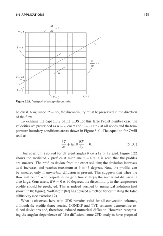
Figure 5.21. Transport of a step discontinuity.

below it. Now, since P =∞, the discontinuity must be preserved in the direction
of the flow.
To examine the capability of the UDS for this large Peclet number case, the
velocities are prescribed as u = U cosθ and v = U sinθ at all nodes and the tem-
perature boundary conditions are as shown in Figure 5.21. The equation for T will
read as
∂T ∂T
+ tanθ = 0. (5.131)
∂x ∂y
This equation is solved for different angles θ ona12 × 12 grid. Figure 5.22
shows the predicted T profiles at midplane x = 0.5. It is seen that the profiles
are smeared. The profiles deviate from the exact solution; the deviation increases
as θ increases and reaches maximum at θ = 45 degrees. Now, the profiles can
be smeared only if numerical diffusion is present. This suggests that when the
flow inclination with respect to the grid line is large, the numerical diffusion is
also large. Conversely, if θ = 0 or 90 degrees, the discontinuity in the temperature
profile should be predicted. This is indeed verified by numerical solutions (not
shown in the figure). Wolfshtein [89] has devised a method for estimating the false
diffusivity (see exercise 12).
What is observed here with UDS remains valid for all convection schemes,
although the profile-shape-sensing CONDIF and TVD schemes demonstrate re-
duced deviations and, therefore, reduced numerical diffusion. However, recognis-
ing the angular dependence of false diffusion, some CFD analysts have proposed