Page 173 - Introduction to Computational Fluid Dynamics

P1: IWV
May 20, 2005
12:28
CB908/Date
0521853265c05
152
1.0 0 521 85326 5 2D CONVECTION – CARTESIAN GRIDS
EXACT
0.8

0.6
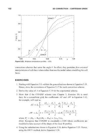
T (0.5, Y) 0.4

0.2 30
45 Θ = 15

EXACT
0.0
0.00 0.25 0.50 0.75 1.00
Y
Figure 5.22. Midplane temperature profiles – UDS.

convection schemes that sense the angle θ. In effect, they postulate flow-oriented
interpolations of cell-face values rather than use the nodal values straddling the cell
faces.

EXERCISES
1. Starting with Equation 5.8, validate the generalisations shown in Equation 5.19.
Hence, show the correctness of Equation 5.17 for each convection scheme.
2. Derive the value of A in Equation 5.19 for the exponential scheme.

3. Show that if the CONDIF scheme (see Chapter 3, Exercise 10) is used
then, for a nonuniform grid, the coefficients AE and AW in Equation 5.12,
for example, will read as

|P c e |− P c e d w |P c w |− P c w
AE = d e 1 + + ,
4 R ∗ 4
x

|P c w |+ P c w |P c e |+ P c e
AW = d w 1 + + d e R ∗ x ,
4 4
where R = ( E − P )/( P − W ) × x w / x e .
∗
x
(Hint: Recognise that CONDIF is essentially a CDS whose coefficients are
modified to take account of the shape of the local profile).
4. Using the substitutions shown in Equation 5.24, derive Equation 5.25. Hence,
using the IOCV method, derive Equation 5.28.