Page 177 - Introduction to Computational Fluid Dynamics

P1: IWV
0 521 85326 5
May 20, 2005
12:28
0521853265c05
CB908/Date
156
X 2 2D CONVECTION – CARTESIAN GRIDS
DUCT
BOUNDARY
2B X 1

2A

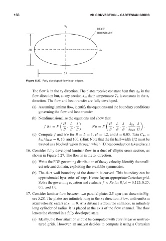
Figure 5.27. Fully developed flow in an ellipse.

The flow is in the x 3 direction. The plates receive constant heat flux q w in the
flow direction but, at any section x 3 , their temperature T w is constant in the x 1
direction. The flow and heat transfer are fully developed.
(a) Assuming laminar flow, identify the equations and the boundary conditions
governing the flow and heat transfer

(b) Nondimensionalise the equations and show that

H L δ H L δ k fin δ
fRe = F , , , Nu = F , , , .
B B B B B B k fluid H
(c) Compute f and Nu for B = L = 1, H = 1.2, and δ = 0.05. Take C fin =
k fin /k fluid = 0, 10, and 100. (Hint: Note that the fin half-width δ/2 must be
treated as a blocked region through which 1D heat conduction takes place.)
16. Consider fully developed laminar flow in a duct of elliptic cross section, as
shown in Figure 5.27. The flow is in the x 3 direction.
(a) Write the PDE governing distribution of the u 3 velocity. Identify the small-
est relevant domain, exploiting the available symmetries.
(b) The duct wall boundary of the domain is curved. This boundary can be
approximated by a series of steps. Hence, lay an appropriate Cartesian grid.
Solve the governing equation and evaluate f × Re for B/A = 0.125, 0.25,
0.5, and 1.0.
17. Consider laminar flow between two parallel plates 2B apart, as shown in Fig-
ure 5.28. The plates are infinitely long in the x 3 direction. Flow, with uniform
axial velocity, enters at x 1 = 0. At a distance S from the entrance, an infinitely
long cylinder of radius R is placed at the axis of the flow channel. The flow
leaves the channel in a fully developed state.
(a) Ideally, the flow situation should be computed with curvilinear or unstruc-
tured grids. However, an analyst decides to compute it using a Cartesian