Page 234 - Introduction to Mineral Exploration

10: EVALUATION TECHNIQUES 217

available in all exploration offices and must be being outside the range is higher – four chances
read and understood. Samplers should rarely, in 20 or quadruple the previous calculation.
if ever, work alone and visits to mine work- Commonsense must be used in the inter-
ings (surface or underground) should be accom- pretation of the results of any sampling pro-
panied. Visits to abandoned mine workings gram and particularly with the problem of
need particular care and the workings should re-sampling in order to increase the n statistic.
be assessed fully for potential weak rock As an example, a zinc prospect 200 km from
conditions, weak roof support, water extent, the nearest road or railway is sampled and
noxious gases, and other hazards before samp- preliminary estimates are 2.1% zinc with an
ling commences. estimated overall reserve tonnage of about
200,000 t. There is no point in sharpening this
grade estimate by taking more samples as the
After sampling
low tonnage, approximate grade and location
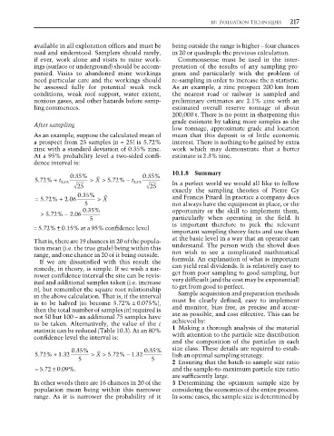
As an example, suppose the calculated mean of mean that this deposit is of little economic
a prospect from 25 samples (n = 25) is 5.72% interest. There is nothing to be gained by extra
zinc with a standard deviation of 0.35% zinc. work which may demonstrate that a better
At a 95% probability level a two-sided confi- estimate is 2.3% zinc.
dence interval is:
10.1.8 Summary
.
.
035% 035%
>
>
Y
.
572% + t 25.% . 25.% In a perfect world we would all like to follow
572% − t
25 25 exactly the sampling theories of Pierre Gy
. 035 %
.
= 572 % + 2 .06 > Y and Francis Pitard. In practice a company does
5 not always have the equipment in place, or the
. 035 % opportunity or the skill to implement them,
.
> 572 % − 2 .06
5 particularly when operating in the field. It
is important therefore to pick the relevant
= 5.72% ± 0.15% at a 95% confidence level
important sampling theory facts and use them
at the basic level in a way that an operator can
That is, there are 19 chances in 20 of the popula-
tion mean (i.e. the true grade) being within this understand. The person with the shovel does
range, and one chance in 20 of it being outside. not wish to see a complicated mathmatical
If we are dissatisfied with this result the formula. An explanation of what is important
remedy, in theory, is simple. If we wish a nar- can yield real dividends. It is relatively easy to
rower confidence interval the site can be revis- get from poor sampling to good sampling, but
ited and additional samples taken (i.e. increase very difficuilt (and the cost may be exponential)
n), but remember the square root relationship to get from good to perfect.
in the above calculation. That is, if the interval Sample acquisition and preparation methods
is to be halved (to become 5.72% ± 0.075%), must be clearly defined, easy to implement
then the total number of samples (n) required is and monitor, bias free, as precise and accur-
not 50 but 100 – an additional 75 samples have ate as possible, and cost effective. This can be
to be taken. Alternatively, the value of the t achieved by:
statistic can be reduced (Table 10.3). At an 80% 1 Making a thorough analysis of the material
confidence level the interval is: with attention to the particle size distribution
and the composition of the particles in each
035% 035% size class. These details are required to estab-
.
.
572% + 1 32 > Y > 572% − 1 32 lish an optimal sampling strategy.
.
.
.
.
5 5 2 Ensuring that the batch-to-sample size ratio
= 5.72 ± 0.09%. and the sample-to-maximum particle size ratio
are sufficiently large.
In other words there are 16 chances in 20 of the 3 Determining the optimum sample size by
population mean being within this narrower considering the economics of the entire process.
range. As it is narrower the probability of it In some cases, the sample size is determined by