Page 236 - Marks Calculation for Machine Design

P1: Shibu/Sanjay
January 4, 2005
14:35
Brown˙C05
Brown.cls
218
STRENGTH OF MACHINES
However, as the rotation is clockwise the principal stress angle (φ p ) will be negative.
Changing the sign on (tan 2φ p ) and solving for angle (φ p ) gives a value that is very close
to the value found in Example 5 in Sec. 5.2, that is (−15.7 ).
◦
tan 2φ p =−0.612
2φ p =−31.4 ◦
φ p =−15.7 ◦
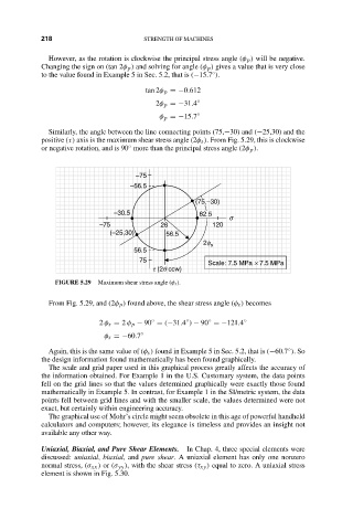
Similarly, the angle between the line connecting points (75,−30) and (−25,30) and the
positive (τ) axis is the maximum shear stress angle (2φ s ). From Fig. 5.29, this is clockwise
or negative rotation, and is 90 more than the principal stress angle (2φ p ).
◦
–75
–56.5
(75,–30)
–30.5 82.5
s
–75 26 120
(–25,30) 56.5
2f s
56.5
75
Scale: 7.5 MPa ¥ 7.5 MPa
t (2q ccw)
FIGURE 5.29 Maximum shear stress angle (φ s ).

From Fig. 5.29, and (2φ p ) found above, the shear stress angle (φ s ) becomes

◦
◦
◦
2 φ s = 2 φ p − 90 = (−31.4 ) − 90 =−121.4 ◦
φ s =−60.7 ◦
Again, this is the same value of (φ s ) found in Example 5 in Sec. 5.2, that is (−60.7 ).So
◦
the design information found mathematically has been found graphically.
The scale and grid paper used in this graphical process greatly affects the accuracy of
the information obtained. For Example 1 in the U.S. Customary system, the data points
fell on the grid lines so that the values determined graphically were exactly those found
mathematically in Example 5. In contrast, for Example 1 in the SI/metric system, the data
points fell between grid lines and with the smaller scale, the values determined were not
exact, but certainly within engineering accuracy.
The graphical use of Mohr’s circle might seem obsolete in this age of powerful handheld
calculators and computers; however, its elegance is timeless and provides an insight not
available any other way.

Uniaxial, Biaxial, and Pure Shear Elements. In Chap. 4, three special elements were
discussed: uniaxial, biaxial, and pure shear. A uniaxial element has only one nonzero
normal stress, (σ xx ) or (σ yy ), with the shear stress (τ xy ) equal to zero. A uniaxial stress
element is shown in Fig. 5.30.