Page 203 - Materials Science and Engineering An Introduction

6.3 Stress–Strain Behavior • 175

2

= Tangent modulus (at )

2
Unload
1
Stress Slope = modulus Stress
of elasticity

= Secant modulus
Load (between origin and )

1
0
0
Strain
Figure 6.5 Schematic
stress–strain diagram Strain
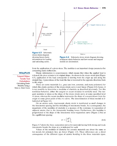
showing linear elastic Figure 6.6 Schematic stress–strain diagram showing
deformation for loading nonlinear elastic behavior and how secant and tangent
and unloading cycles. moduli are determined.

from the application of a given stress. The modulus is an important design parameter for
computing elastic deflections.
Elastic deformation is nonpermanent, which means that when the applied load is
released, the piece returns to its original shape. As shown in the stress–strain plot (Figure
Tutorial Video: 6.5), application of the load corresponds to moving from the origin up and along the
Tensile Test
Calculations straight line. Upon release of the load, the line is traversed in the opposite direction, back
to the origin.
Calculating Elastic There are some materials (i.e., gray cast iron, concrete, and many polymers) for
Modulus Using a which this elastic portion of the stress–strain curve is not linear (Figure 6.6); hence, it
Stress vs. Strain Curve
is not possible to determine a modulus of elasticity as described previously. For this
nonlinear behavior, either the tangent or secant modulus is normally used. The tan-
gent modulus is taken as the slope of the stress–strain curve at some specified level
of stress, whereas the secant modulus represents the slope of a secant drawn from the
origin to some given point of the s-P curve. The determination of these moduli is il-
lustrated in Figure 6.6.
On an atomic scale, macroscopic elastic strain is manifested as small changes in
the interatomic spacing and the stretching of interatomic bonds. As a consequence, the
magnitude of the modulus of elasticity is a measure of the resistance to separation of
adjacent atoms, that is, the interatomic bonding forces. Furthermore, this modulus is
proportional to the slope of the interatomic force–separation curve (Figure 2.10a) at
the equilibrium spacing:

dF
E a b (6.6)
dr
r 0
Figure 6.7 shows the force–separation curves for materials having both strong and weak
interatomic bonds; the slope at r 0 is indicated for each.
Values of the modulus of elasticity for ceramic materials are about the same as
for metals; for polymers they are lower (Figure 1.5). These differences are a direct
consequence of the different types of atomic bonding in the three materials types.