Page 505 - Mathematical Techniques of Fractional Order Systems

492 Mathematical Techniques of Fractional Order Systems

(A) (B)
1.6 1.5
1.4
1
1.2
0.5
1
y z
0.8
0
0.6
−0.5
0.4
0.2 −1
−1.5 −1 −0.5 0 0.5 1 1.5 −2 −1 0 1 2
x x
(C)
1.5
1

0.5
z
0
−0.5
−1
0 0.5 1 1.5
y
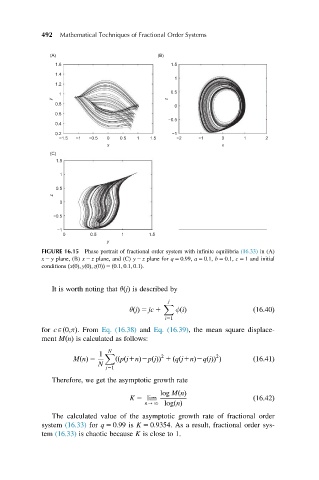
FIGURE 16.15 Phase portrait of fractional order system with infinite equilibria (16.33) in (A)
x 2 y plane, (B) x 2 z plane, and (C) y 2 z plane for q 5 0:99, a 5 0:1, b 5 0:1, c 5 1 and initial
conditions ðxð0Þ; yð0Þ; zð0ÞÞ 5 ð0:1; 0:1; 0:1Þ.

It is worth noting that θ jðÞ is described by
j
X
θðjÞ 5 jc 1 φðiÞ ð16:40Þ
i51
for cAð0;πÞ. From Eq. (16.38) and Eq. (16.39), the mean square displace-
ment MðnÞ is calculated as follows:
N
1 X 2 2
MðnÞ 5 ððpðj1nÞ2pðjÞÞ 1 ðqðj1nÞ2qðjÞÞ Þ ð16:41Þ
N
j51
Therefore, we get the asymptotic growth rate
log MðnÞ
K 5 lim ð16:42Þ
n-N logðnÞ
The calculated value of the asymptotic growth rate of fractional order
system (16.33) for q 5 0:99 is K 5 0:9354. As a result, fractional order sys-
tem (16.33) is chaotic because K is close to 1.