Page 68 - Mathematical Techniques of Fractional Order Systems

Nonlinear Fractional Order Boundary-Value Problems Chapter | 2 57

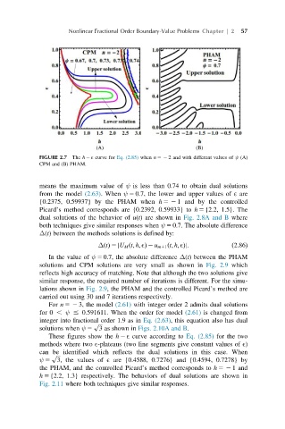
FIGURE 2.7 The h 2 E curve for Eq. (2.85) when n 52 2 and with different values of ψ (A)
CPM and (B) PHAM.

means the maximum value of ψ is less than 0.74 to obtain dual solutions
from the model (2.63). When ψ 5 0.7, the lower and upper values of E are
{0.2375, 0.59937} by the PHAM when h 52 1 and by the controlled
Picard’s method corresponds are {0.2392, 0.59933} to h 5 {2.2, 1.5}. The
dual solutions of the behavior of u(t) are shown in Fig. 2.8A and B where
both techniques give similar responses when ψ 5 0.7. The absolute difference
Δ(t) between the methods solutions is defined by:
ΔðtÞ 5 jU M ðt; h; EÞ 2 u m11 ðt; h; EÞj: ð2:86Þ
In the value of ψ 5 0.7, the absolute difference Δ(t) between the PHAM
solutions and CPM solutions are very small as shown in Fig. 2.9 which
reflects high accuracy of matching. Note that although the two solutions give
similar response, the required number of iterations is different. For the simu-
lations shown in Fig. 2.9, the PHAM and the controlled Picard’s method are
carried out using 30 and 7 iterations respectively.
For n 52 3, the model (2.61) with integer order 2 admits dual solutions
for 0 , ψ # 0.591611. When the order for model (2.61) is changed from
integer into fractional order 1.9 as in Eq. (2.63), this equation also has dual
p ffiffiffi
solutions when ψ 5 3 as shown in Figs. 2.10A and B.
These figures show the h 2 E curve according to Eq. (2.85) for the two
methods where two E-plateaus (two line segments give constant values of E)
can be identified which reflects the dual solutions in this case. When
p ffiffiffi
ψ 5 3, the values of E are {0.4588, 0.7276} and {0.4594, 0.7278} by
the PHAM, and the controlled Picard’s method corresponds to h 52 1 and
h 5 {2.2, 1.3} respectively. The behaviors of dual solutions are shown in
Fig. 2.11 where both techniques give similar responses.