Page 69 - Mathematical Techniques of Fractional Order Systems

58 Mathematical Techniques of Fractional Order Systems

1.0 1.0
Upper solution
ψ = 0.67, 0.7, 0.73
0.8 0.8
Upper solution
u(t) 0.6 u(t) 0.6 PHAM
CPM
0.4 Lower solution n = –2
n = –2 0.4 M = 30
Lower solution ψ = 0.67
0.2 m = 6
0.2
0.0 0.2 0.4 0.6 0.8 1.0
0.0 0.2 0.4 0.6 0.8 1.0
t t
(A) (B)
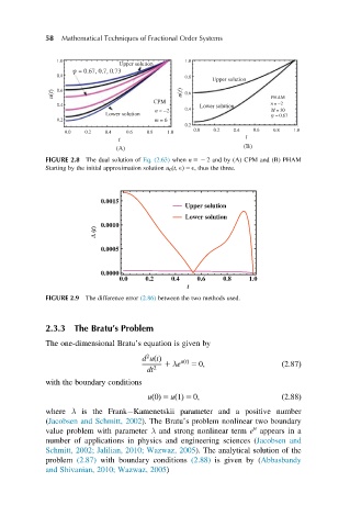
FIGURE 2.8 The dual solution of Eq. (2.63) when n 52 2 and by (A) CPM and (B) PHAM
Starting by the initial approximation solution u 0 (t, E) 5 E, thus the three.

0.0015
Upper solution
Lower solution
0.0010
Δ (t)

0.0005

0.0000
0.0 0.2 0.4 0.6 0.8 1.0
t
FIGURE 2.9 The difference error (2.86) between the two methods used.

2.3.3 The Bratu’s Problem
The one-dimensional Bratu’s equation is given by
2
d uðtÞ
1 λe uðtÞ 5 0; ð2:87Þ
dt 2
with the boundary conditions
uð0Þ 5 uð1Þ 5 0; ð2:88Þ

where λ is the Frank Kamenetskii parameter and a positive number
(Jacobsen and Schmitt, 2002). The Bratu’s problem nonlinear two boundary
u
value problem with parameter λ and strong nonlinear term e appears in a
number of applications in physics and engineering sciences (Jacobsen and
Schmitt, 2002; Jalilian, 2010; Wazwaz, 2005). The analytical solution of the
problem (2.87) with boundary conditions (2.88) is given by (Abbasbandy
and Shivanian, 2010; Wazwaz, 2005)