Page 73 - Mathematical Techniques of Fractional Order Systems

62 Mathematical Techniques of Fractional Order Systems

20

α = 1.8
α = 1.9
15 α = 2
α = 2 Exact

10
∋

5

0
0.0 0.5 1.0 1.5 2.0 2.5 3.0 3.5
λ
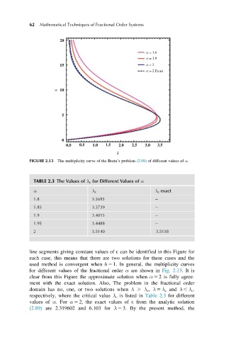
FIGURE 2.13 The multiplicity curve of the Bratu’s problem (2.90) of different values of α.

TABLE 2.3 The Values of λ c for Different Values of α

α λ c λ c exact
1.8 3.3693
1.85 3.3739
1.9 3.4015
1.95 3.4488
2 3.5140 3.5138

line segments giving constant values of E can be identified in this Figure for
each case, this means that there are two solutions for these cases and the
used method is convergent when h 5 1. In general, the multiplicity curves
for different values of the fractional order α are shown in Fig. 2.13.It is
clear from this Figure the approximate solution when α 5 2 is fully agree-
ment with the exact solution. Also, The problem in the fractional order
domain has no, one, or two solutions when λ . λ c , λ 5 λ c and λ , λ c .
respectively, where the critical value λ c is listed in Table 2.3 for different
values of α. For α 5 2, the exact values of E from the analytic solution
(2.89) are 2.319602 and 6.103 for λ 5 3. By the present method, the