Page 76 - Mathematical Techniques of Fractional Order Systems

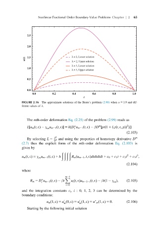
Nonlinear Fractional Order Boundary-Value Problems Chapter | 2 65

2.5

2.0

u(t) 1.5 λ = 2, Lower solution
λ = 2, Upper solution
λ = 3, Lower solution
1.0
λ = 3, Upper solution

0.5

0.0
0.0 0.2 0.4 0.6 0.8 1.0
t
FIGURE 2.16 The approximate solutions of the Bratu’s problem (2.90) when α 5 1.9 and dif-
ferent values of λ.

The mth-order deformation Eq. (2.25) of the problem (2.99) reads as
α m 2
L½u m ðt; EÞ 2 χ u m21 ðt; Eފ 5 hfD u m21 ðt; EÞ 2 βD ½ptð1 1 ðϕðt; E; pÞÞ ÞŠg
m
t
ð2:103Þ
4
@
By selecting L 5 @t 4 and using the properties of homotopy derivative D m
(2.7) thus the explicit form of the mth-order deformation Eq. (2.103) is
given by
ðð ðð
2
3
u m ðt; EÞ 5 χ u m21 ðt; EÞ 1 h R m ðu m21 ; t; EÞdtdtdtdt 1 c 0 1 c 1 t 1 c 2 t 1 c 3 t ;
m
ð2:104Þ
where
m21
α X
R m 5 D u m21 ðt; EÞ 2 βt u i ðt; EÞu m212i ðt; EÞ 2 βtð1 2 χ Þ; ð2:105Þ
t m
i50
and the integration constants c i , i : 0, 1, 2, 3 can be determined by the
boundary conditions:
0
u m ð1; EÞ 5 u ð0; EÞ 5 u ð1; EÞ 5 uv m ð1; EÞ 5 0: ð2:106Þ
0
m m
Starting by the following initial solution