Page 75 - Mathematical Techniques of Fractional Order Systems

64 Mathematical Techniques of Fractional Order Systems

TABLE 2.4 The Numerical Solutions of Eq. (2.90) for Different Values of α
Lower solution Upper solution

t α 5 2 α 5 1.9 α 5 1.8 α 5 2 α 5 1.9 α 5 1.8
0.1 0.2157 0.2406 0.2607 0.5919 0.6037 0.6573
0.2 0.3943 0.43498 0.4645 1.1284 1.1375 1.2224
0.3 0.5284 0.57644 0.60665 1.571 1.558 1.6401
0.4 0.6118 0.65929 0.68304 1.8693 1.8131 1.8512
0.5 0.6401 0.6805 0.69319 1.9755 1.8646 1.8318
0.6 0.6118 0.64097 .64133 1.8691 1.7133 1.6154
0.7 0.5284 0.54504 0.53564 1.5708 1.4 1.2702
0.8 0.3943 0.4004 0.38652 1.1283 0.9808 0.8601
0.9 0.2157 0.21568 0.2047 0.5919 0.50342 0.42861

2.0

1.5
α = 2, Lower solution
α = 2, Upper solution
α = 1.8, Lower solution
u(t) 1.0 α = 1.8, Upper solution

0.5

0.0
0.0 0.2 0.4 0.6 0.8 1.0
t
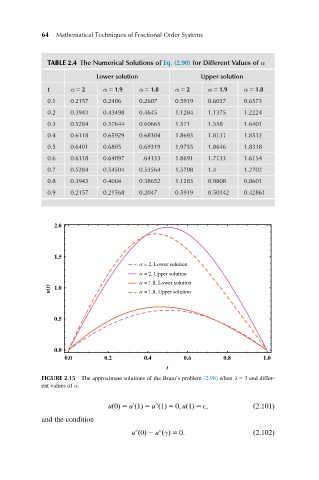
FIGURE 2.15 The approximate solutions of the Bratu’s problem (2.90) when λ 5 3 and differ-
ent values of α.

uð0Þ 5 u ð1Þ 5 uvð1Þ 5 0; uð1Þ 5 E; ð2:101Þ
0
and the condition
uvð0Þ 2 uvðγÞ 5 0: ð2:102Þ