
Page 70 - Mathematical Techniques of Fractional Order Systems
P. 70
Nonlinear Fractional Order Boundary-Value Problems Chapter | 2 59
p ffiffiffi
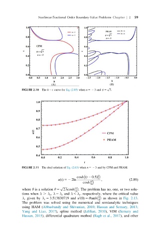
FIGURE 2.10 The h 2 E curve for Eq. (2.85) when n 52 3 and ψ 5 3.
1.0
0.9
0.8
0.7
u(t) CPM
0.6
PHAM
0.5
0.4
0.0 0.2 0.4 0.6 0.8 1.0
t
FIGURE 2.11 The dual solution of Eq. (2.63) when n 52 3 and by CPM and PHAM.
θ
cosh ðt 2 0:5Þ 2
uðtÞ 52 2ln ; ð2:89Þ
cosh θ
4
p ffiffiffiffiffiffi
where θ is a solution θ 5 2λcosh θ . The problem has no, one, or two solu-
4
tions when λ . λ c , λ 5 λ c and λ , λ c . respectively, where the critical value
θ
λ c given by λ c 5 3.513830719 and u ð0Þ 5 θtanh as shown in Fig. 2.13.
0
4
The problem was solved using the numerical and semianalytic techniques
using HAM (Abbasbandy and Shivanian, 2010; Hassan and Semary, 2013;
Yang and Liao, 2017), spline method (Jalilian, 2010), VIM (Semary and
Hassan, 2015), differential quadrature method (Ragb et al., 2017), and other