
Page 72 - Mathematical Techniques of Fractional Order Systems
P. 72
Nonlinear Fractional Order Boundary-Value Problems Chapter | 2 61
(2.91) which can be used to obtain the mth-successive approximations (2.96).
The first approximation solution u 1 (t, h, E) is given by:
α
α
0:033ht λ ht λ
u 1 ðt; h; EÞ 5 tE 2 2 f 1 1 f 2 1 f 3 1 f 4 1 f 5 1 f 6 1 f 7 1 f 8 1 f 9
Γ½α Γ½α
α
α
t λ ht λ t 11α Eλ ht 1:1α Eλ
2 1 2 1
Γ½1 1 α Γ½1 1 α Γ½2 1 α Γ½2 1 α
ð2:97Þ
where,
20:105α10:1tE2 e 22:30α t α λ 2 0:1e 22:30α t 1:1α Eλ
f 1 5 0:1481e Γ½11α Γ½11α ;-
f 2 5 0:083e 20:223α10:2tE2 e 21:60α t α λ 2 0:2e 21:609α t 1:1α Eλ ;
Γ½21α
Γ½11α
20:356α10:3tE2 e 21:20α t α λ 2 0:3e 21:203α t 1:1α Eλ
f 3 5 0:190e Γ½11α Γ½11α ;-
20:510α10:4tE2 e 20:916α t α λ 2 0:4e 20:916α t 1:1α Eλ
f 4 5 0:111e Γ½1:1α Γ½2:1α ;
f 5 5 0:266e 20:693α10:5tE2 e 20:693α t α λ 2 0:5e 20:69α t 1:1α Eλ ;
Γ½11α
Γ½21α
f 6 5 0:166e 20:916α10:6tE2 e 20:510α t α λ 2 0:6e 20:510α t 1:1α Eλ ;
Γ½21α
Γ½1:1α
21:203α10:7tE2 e 20:35α t α λ 2 0:7e 20:356α t 1:1α Eλ
f 7 5 0:444e Γ½11α Γ½21α ;
21:609α10:8tE2 e 20:223α t α λ 2 0:8e 20:223α t 1:1α Eλ
f 8 5 0:33e Γ½1:1α Γ½2:1α ;
f 9 5 1:333e 22:302α10:9tE2 e 20:1053α t α λ 2 0:899e 20:1053α t 1:1α Eλ ; and so on. With the help of
Γ½2:1α
Γ½1:1α
forcing condition u(1) 5 0, then
uð1Þ 5 u m11 ð1; E; hÞ 5 0: ð2:98Þ
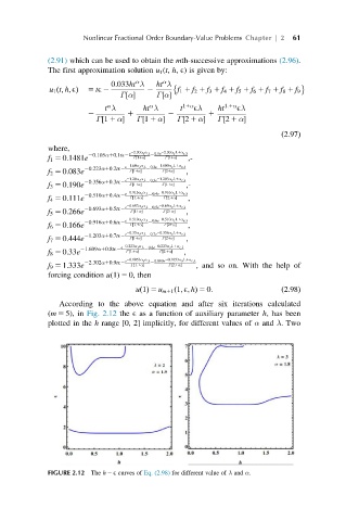
According to the above equation and after six iterations calculated
(m 5 5), in Fig. 2.12 the E as a function of auxiliary parameter h, has been
plotted in the h range [0, 2] implicitly, for different values of α and λ. Two
FIGURE 2.12 The h 2 E curves of Eq. (2.98) for different value of λ and α.