Page 235 - Matrix Analysis & Applied Linear Algebra

230 Chapter 4 Vector Spaces
b
p(t) (t m ,b m ) •
ε m

•
t m ,p (t m ) •
(t 2 ,b 2 ) •
ε 2 •
•
•
t 2 ,p (t 2 ) •
t
•
•

• t 1 ,p (t 1 )
ε 1

• (t 1 ,b 1 )

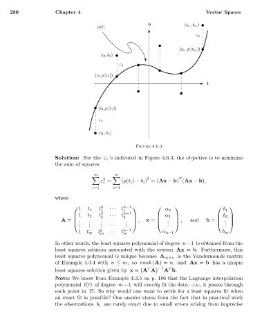
Figure 4.6.3
Solution: For the ε i ’s indicated in Figure 4.6.3, the objective is to minimize
the sum of squares
m m
2 2 T
ε = (p(t i ) − b i ) =(Ax − b) (Ax − b),
i
i=1 i=1
where

1 t 1 t 1 ··· t 1 α 0 b 1
 2 n−1     
 1 t 2 t 2 2 ··· t n−1   α 1   b 2 
2
A =  . . . .  , x =  .  , and b =  .  .
 . . . . .
. . . ··· .   .   . 
.
1 t 2 ··· t n−1 α n−1 b m
t m
m m
In other words, the least squares polynomial of degree n−1 is obtained from the
least squares solution associated with the system Ax = b. Furthermore, this
least squares polynomial is unique because A m×n is the Vandermonde matrix
of Example 4.3.4 with n ≤ m, so rank (A)= n, and Ax = b has a unique
T
T
least squares solution given by x = A A −1 A b.

Note: We know from Example 4.3.5 on p. 186 that the Lagrange interpolation
polynomial (t) of degree m−1 will exactly fit the data—i.e., it passes through
each point in D. So why would one want to settle for a least squares fit when
an exact fit is possible? One answer stems from the fact that in practical work
the observations b i are rarely exact due to small errors arising from imprecise