Page 236 - Matrix Analysis & Applied Linear Algebra

4.6 Classical Least Squares 231

measurements or from simplifying assumptions. For this reason, it is the trend
of the observations that needs to be fitted and not the observations themselves.
To hit the data points, the interpolation polynomial (t) is usually forced to
oscillate between or beyond the data points, and as m becomes larger the oscil-
lations can become more pronounced. Consequently, (t) is generally not useful
in making estimations concerning the trend of the observations—Example 4.6.3
drives this point home. In addition to exactly hitting a prescribed set of data
points, an interpolation polynomial called the Hermite polynomial (p. 607) can
be constructed to have specified derivatives at each data point. While this helps,
it still is not as good as least squares for making estimations on the basis of
observations.

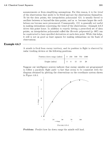
Example 4.6.3
A missile is fired from enemy territory, and its position in flight is observed by
radar tracking devices at the following positions.

Position down range (miles) 0 250 500 750 1000
Height (miles) 0 8 15 19 20

Suppose our intelligence sources indicate that enemy missiles are programmed
to follow a parabolic flight path—a fact that seems to be consistent with the
diagram obtained by plotting the observations on the coordinate system shown
in Figure 4.6.4.
20

15

10
b = Height

5

0
0 250 500 750 1000
t = Range
Figure 4.6.4
Problem: Predict how far down range the missile will land.