Page 238 - Matrix Analysis & Applied Linear Algebra

4.6 Classical Least Squares 233

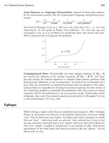
Least Squares vs.Lagrange Interpolation. Instead of using least squares,
fit the observations exactly with the fourth-degree Lagrange interpolation poly-
nomial
11 17 2 1 3 1 4
(t)= t + t − t + t
375 750000 18750000 46875000000
described in Example 4.3.5 on p. 186 (you can verify that (t i )= b i for each
observation). As the graph in Figure 4.6.5 indicates, (t) has only one real
nonnegative root, so it is worthless for predicting where the missile will land.
This is characteristic of Lagrange interpolation.

y = (t)

Figure 4.6.5

Computational Note: Theoretically, the least squares solutions of Ax = b
T
T
are exactly the solutions of the normal equations A Ax = A b, but form-
ing and solving the normal equations to compute least squares solutions with
floating-point arithmetic is not recommended. As pointed out in Example 4.5.1
on p. 214, any sensitivities to small perturbations that are present in the under-
lying problem are magnified by forming the normal equations. In other words, if
the underlying problem is somewhat ill-conditioned, then the system of normal
equations will be ill-conditioned to an even greater extent. Numerically stable
techniques that avoid the normal equations are presented in Example 5.5.3 on
p. 313 and Example 5.7.3 on p. 346.

Epilogue

While viewing a region in the Taurus constellation on January 1, 1801, Giuseppe
Piazzi, an astronomer and director of the Palermo observatory, observed a small
“star” that he had never seen before. As Piazzi and others continued to watch
this new “star”—which was really an asteroid—they noticed that it was in fact
moving, and they concluded that a new “planet” had been discovered. However,
their new “planet” completely disappeared in the autumn of 1801. Well-known
astronomers of the time joined the search to relocate the lost “planet,” but all
efforts were in vain.