Page 234 - Matrix Analysis & Applied Linear Algebra

4.6 Classical Least Squares 229

The famous Gauss–Markov theorem (developed on p. 448) states that under
certain reasonable assumptions concerning the random error function ε, the
“best” estimates for the α i ’s are obtained by minimizing the sum of squares
T
(Ax − b) (Ax − b). In other words, the least squares estimates are the “best”
way to estimate the α i ’s.
Returning to our ice cream example, it can be verified that b /∈ R (A), so, as
expected, the system Ax = b is not consistent, and we cannot determine exact
values for α 0 ,α 1 , and α 2 . The best we can do is to determine least squares esti-
T
T
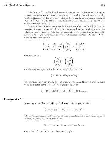
mates for the α i ’s by solving the associated normal equations A Ax = A b,
which in this example are
     
9 18 −45 α 0 1.79
18 42 −90 = 3.73 .
   α 1   
−45 −90 375 α 2 −8.2
The solution is
   
α 0 .174
 α 1  =  .025  ,
α 2 .005
and the estimating equation for mean weight loss becomes

ˆ y = .174 + .025t 1 + .005t 2 .

For example, the mean weight loss of a pint of ice cream that is stored for nine
o
weeks at a temperature of −35 F is estimated to be
ˆ y = .174 + .025(9) + .005(−35) = .224 grams.

Example 4.6.2
Least Squares Curve Fitting Problem: Find a polynomial

2
p(t)= α 0 + α 1 t + α 2 t + ··· + α n−1 t n−1

with a specified degree that comes as close as possible in the sense of least squares
to passing through a set of data points

D = {(t 1 ,b 1 ), (t 2 ,b 2 ),. . . , (t m ,b m )} ,

where the t i ’s are distinct numbers, and n ≤ m.