Page 276 - Mechanical design of microresonators _ modeling and applications

0-07-145538-8_CH05_275_08/30/05

Resonant Micromechanical Systems

Resonant Micromechanical Systems 275
3. Resonance in both the drive and sense branches: Ȧ d = Ȧ d,r = Ȧ s,r . in
this particular case (the corresponding design is known as the well-
tuned gyroscope), the drive and sense branches are identical in terms
of both stiffness and damping, and ȕ d = ȕ s = 1. In addition, the driving
frequency is equal to the resonant frequencies about the x and y
directions. The sense amplitude of Eq. (5.126) becomes
ȦF 0
Y =
ds 3 (5.130)
2ȟ ȟ mȦ
d s d,r
and definitely the sense amplitude is maximized.
As Eqs. (5.126), (5.128), (5.129), and (5.130) indicate, the external
angular velocity Ȧ can be determined in either of the four design cases
in terms of the system’s design parameters and assuming the sense
displacement can be measured (which is most often performed by ca-
pacitive means in commercially available microfabricated gyroscopes).

Example: Compare the drive-resonance and sense-resonance sense ampli-
tudes in the case where damping properties are identical for the drive and
sense branches.
When the damping properties are identical for the drive and sense
branches, Eqs. (5.128) and (5.129) can be combined into

2 2
Y ȕ (1 íȕ ) + (2 ȟȕ ) 2
d = s d d (5.131)
Y ȕ (1 íȕ ) + (2 ȟȕ ) 2
2 2
s d s s
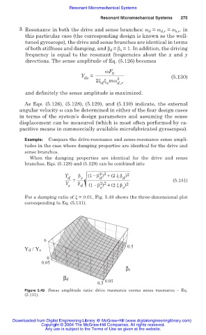
For a damping ratio of ȟ = 0.01, Fig. 5.49 shows the three-dimensional plot
corresponding to Eq. (5.131).

6
0.5
Yd / Ys
0
0.05
βs
βd
0.5 0.05
Figure 5.49 Sense amplitude ratio: drive resonance versus sense resonance – Eq.
(5.131).

Downloaded from Digital Engineering Library @ McGraw-Hill (www.digitalengineeringlibrary.com)
Copyright © 2004 The McGraw-Hill Companies. All rights reserved.
Any use is subject to the Terms of Use as given at the website.