Page 281 - Mechanical design of microresonators _ modeling and applications

0-07-145538-8_CH05_280_08/30/05

Resonant Micromechanical Systems

280 Chapter Five
drive axis drive axis

sense axis
sense axis
sense axis
sense axis

drive axis drive axis

input axis input axis

(a) (b)
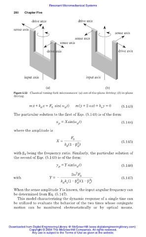
Figure 5.53 Classical tuning-fork microsensors: (a) out-of-the-plane driving; (b) in-plane
driving.

mx ˙˙ + k x = F sin( Ȧ t) m(y ˙˙ +2 Ȧx ˙ ) + k y =0
d 0 d s (5.143)
The particular solution to the first of Eqs. (5.143) is of the form:
x = Xsin(Ȧ t) (5.144)
d
p
where the amplitude is
F 0
X = (5.145)
2
k (1 íȕ )
d
d
with ȕ d being the frequency ratio. Similarly, the particular solution of
the second of Eqs. (5.143) is of the form:
y = Y sin(Ȧ t)
p d (5.146)
2
2Ȧ F 0
with Y = í (5.147)
2
2
k k (1 íȕ )(1 íȕ )
d s
s
d
When the sense amplitude Y is known, the input angular frequency can
be determined from Eq. (5.147).
This model characterizing the dynamic response of a single tine can
be utilized to evaluate the behavior of the two tines whose conjugate
motion can be monitored electrostatically or by optical means.

Downloaded from Digital Engineering Library @ McGraw-Hill (www.digitalengineeringlibrary.com)
Copyright © 2004 The McGraw-Hill Companies. All rights reserved.
Any use is subject to the Terms of Use as given at the website.