Page 33 - Mechanical design of microresonators _ modeling and applications

0-07-145538-8_CH01_32_08/30/05

Design at Resonance of Mechanical Microsystems

32 Chapter One
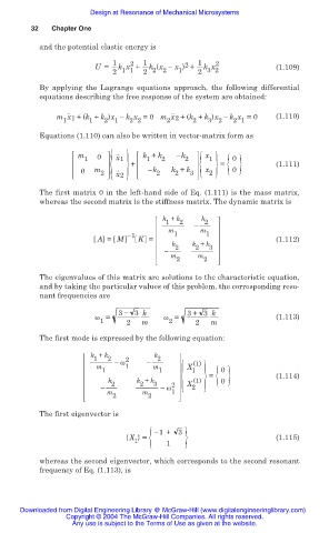
and the potential elastic energy is

1 2 1 1 2
2
U = k x + k (x ෹ x ) + k x (1.109)
2 1 1 2 2 2 1 2 3 2
By applying the Lagrange equations approach, the following differential
equations describing the free response of the system are obtained:
.. ..
m x1 + (k + k )x í k x =0 m x2 + (k + k )x í k x =0 (1.110)
1 1 2 1 2 2 2 2 3 2 2 1
Equations (1.110) can also be written in vector-matrix form as
0 { } + ෹k 2 k + k { x } = { 0} (1.111)
m 1 0 .. x1 k + k 2 ෹k 2 x 1 0
1
..
m
2
2
3
2
x2
The first matrix 0 in the left-hand side of Eq. (1.111) is the mass matrix,
whereas the second matrix is the stiffness matrix. The dynamic matrix is
k + k k
1 2 í 2
m m
í1 1 1
A = M K = (1.112)
k 2 k + k 3
2
෹
m m
2 2
The eigenvalues of this matrix are solutions to the characteristic equation,
and by taking the particular values of this problem, the corresponding reso-
nant frequencies are
3 í 3 k 3+ 3 k
Ȧ = Ȧ = (1.113)
1 2 m 2 2 m
The first mode is expressed by the following equation:

k + k k
1 2 ෹ Ȧ 2 ෹ 2 (1)
m 1 m X
(1) { 0}
1
1
1 3 { X } 0
k 2 k + k = (1.114)
2
෹ ෹ Ȧ 2 2
m m 1
2 2
The first eigenvector is
1 { ෹1+ 3
{X } = 1 } (1.115)
whereas the second eigenvector, which corresponds to the second resonant
frequency of Eq. (1.113), is

Downloaded from Digital Engineering Library @ McGraw-Hill (www.digitalengineeringlibrary.com)
Copyright © 2004 The McGraw-Hill Companies. All rights reserved.
Any use is subject to the Terms of Use as given at the website.