Page 41 - Mechanical design of microresonators _ modeling and applications

0-07-145538-8_CH01_40_08/30/05

Design at Resonance of Mechanical Microsystems

40 Chapter One
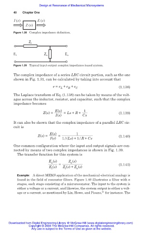
I (s) E (s)
Z (s)

Figure 1.38 Complex impedance definition.

Z i

E i Z o E o

Figure 1.39 Typical input-output complex impedance-based system.

The complex impedance of a series LRC circuit portion, such as the one
shown in Fig. 1.31, can be calculated by taking into account that
e = e + e + e C (1.138)
L
R
The Laplace transform of Eq. (1.138) can be taken by means of the volt-
ages across the inductor, resistor, and capacitor, such that the complex
impedance becomes
E(s) 1
Z(s) = = Ls + R + (1.139)
I(s) Cs

It can also be shown that the complex impedance of a parallel LRC cir-
cuit is
E(s) 1
Z(s) = = (1.140)
I(s) 1 / (Ls) +1 / R + Cs

One common configuration where the input and output signals are con-
nected by means of two complex impedances is shown in Fig. 1.39.
The transfer function for this system is

E (s) Z (s)
o
o
E (s) = Z (s) + Z (s) (1.141)
i i o
Example: A direct MEMS application of the mechanical-electrical analogy is
found in the field of resonator filters. Figure 1.40 illustrates a filter with n
stages, each stage consisting of a microresonator. The input to the system is
either a voltage or a current, and likewise, the system output is either a volt-
21
age or a current, as mentioned by Lin, Howe, and Pisano, for instance. The

Downloaded from Digital Engineering Library @ McGraw-Hill (www.digitalengineeringlibrary.com)
Copyright © 2004 The McGraw-Hill Companies. All rights reserved.
Any use is subject to the Terms of Use as given at the website.