Page 63 - Mechanical Engineers Reference Book

2/4 Electrical and electronics principles

produced by each e.m.f. acting on its own while the other 0
e.m.f.’s are replaced with their respective internal resistances. t
Thevenin’s theorem: The current through a resistor R con-
nected across any two points in an active network is obtained
by dividing the potential difference between the two points,
with R disconnected, by (R + r), where r is the resistance of
the network between the two connection points with R
disconnected and each e.m.f. replaced with its equivalent
internal resistance. An alternative statement of Thevenin’s
theorem is: ‘Any active network can be replaced at any pair of
terminals by an equivalent e.m.f. in series with an equivalent
resistance.’ The more concise version of Thevenin’s theorem is
perhaps a little more indicative of its power in application.
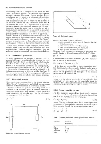
Norton’s theorem: Any active network can be replaced at any Figure 2.2 Electrostatic system
pair of terminals by an equivalent current source in parallel
with an equivalent resistance. It may appear that Norton’s where Q is the total charge in coulombs,
theorem is complementary to Thevenin’s theorem and both so is the permittivity of free space in Faradsim, i.e. the
can be equally well used in the analysis of resistive networks.
field characteristic,
Other useful network analysis techniques include ‘mesh a is the cross-sectional area of the plates,
analysis’, which incorporates Kirchhoff‘s first law, and ‘nodal 1 is the distance separating the plates, and
analysis’, which is based on Kirchhoff‘s second law. Mesh and V is the applied potential difference.
nodal analysis are also essentially complementary techniques. The group (&,,all) is termed the capacitance of the system. It is
usually denoted by C, and is measured in farads (F). Thus
2.1.6 Double-subscript notation Q=C.V (2.14)
To avoid ambiguity in the direction of current, e.m.f. or It is more common to use the microfarad (pF) or the picofarad
potential difference, a double-subscript notation has been (pF) as the unit of measurement.
adopted. Figure 2.1 shows a source of e.m.f. which is acting
from D to A. The e.m.f. is therefore E&. The current flows NB: 1 pF = F: 1 pf = lo-’’ F
from A to B, by traditional convention, and is designated lab.
If the plates are separated by an insulating medium other
From this simple circuit it is apparent that lab = lbc = Zcd = I&. than free space, then these so-called dielectric media have a
The potential difference across the load R is denoted vbc to different value of permittivity. The actual permittivity is
indicate that the potential at B is more positive than that at C. related to the permittivity of free space by the relative
If arrow heads are used to indicate the potential difference, permittivity of the dielectric, i.e.
then they should point towards the more positive potential.
E = Eo ’ E, (2.15)
2.1.7 Electrostatic systems where E, is the relative permittivity of the dielectric. The
permittivity of free space, EO, is numerically equal to
Electrostatic systems are quantified by the physical behaviour (1/36~r) X loM9. The relative permittivity of some of the more
of the ‘charge’. Fortunately, the unified field approach lends common dielectric materials are listed in Table 2.1.
itself well to the quantification of electrostatic systems.
Figure 2.2 shows two parallel, conducting metal plates
separated by an evacuated space. A potential difference is 2.1.8 Simple capacitive circuits
applied across the plates such that they become charged at
equal magnitude but opposite sign. For the electrostatic For three capacitors connected in a simple parallel arrange-
system, equation (2.1) is written ment, the equivalent total capacitance is given as the algebraic
sum of all the capacitances in the circuit, i.e.
eoaV
Q=- (2.13) c = c, + c, + c, (2.16)
1
where C is the total capacitance. For a series capacitance
arrangement of three capacitors, the total equivalent capaci-
A B tance is related through the inverse summation given as
1 1 1 1
- +-+-
--- (2.17)
c c1 cz c3

Table 2.1 Relative permittivities of some typical dielectric materials
Material Relative
permittivity

Air 1
Paper 2-2.5
D C Porcelain 67
Mica 3-7
Figure 2.1 Double-subscript notation