Page 339 - Mechanics of Asphalt Microstructure and Micromechanics

Digital Specimen and Digital T est-Integration of Microstructure into Simulation 331

The simulation model of dynamic modulus test is shown in Figure 10.2b. Due to the
axisymmetric configuration of the macroscopic model, a four-node bilinear axisymmet-
ric solid element with reduced integration and hourglass control was used. The loads
are modeled as distributed boundary traction with sinusoidal repetition (Figure 10.2d)
on the top edge of the sample.

10.2.1.2 Material Model
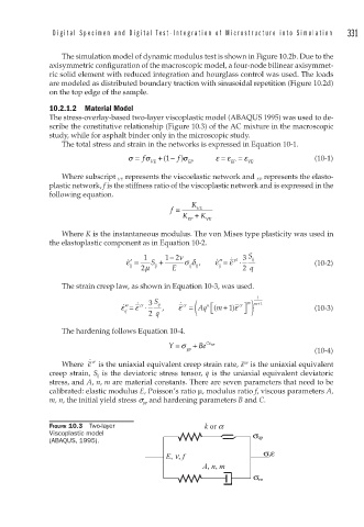
The stress-overlay-based two-layer viscoplastic model (ABAQUS 1995) was used to de-
scribe the constitutive relationship (Figure 10.3) of the AC mixture in the macroscopic
study, while for asphalt binder only in the microscopic study.
The total stress and strain in the networks is expressed in Equation 10-1.
σ = f σ + (1 − f σ ) ε = ε = ε (10-1)
VE EP EP VE
Where subscript VE represents the viscoelastic network and EP represents the elasto-
plastic network, f is the stiffness ratio of the viscoplastic network and is expressed in the
following equation.
K
f = VE
K + K
EP VE
Where K is the instantaneous modulus. The von Mises type plasticity was used in
the elastoplastic component as in Equation 10-2.
− ν
·
⋅
ε · ′ = 1 S + 12 σδ , ε ′′= ε · pl 3 S ij (10-2)
ij μ ij ij ij ij
2 E 2 q
The strain creep law, as shown in Equation 10-3, was used.
(
·
⎤
m m+1
⋅
ε · ′′= ε · cr 3 S ij , ε cr = Aq ( + ε) cr ⎦ ) m 1 (10-3)
n
⎡ m 1
ij ⎣
2 q
The hardening follows Equation 10-4.
Y = σ + Be C EP
ε
yp (10-4)
·
cr
–cr
Where ε is the uniaxial equivalent creep strain rate, e is the uniaxial equivalent
creep strain, S ij is the deviatoric stress tensor, q is the uniaxial equivalent deviatoric
stress, and A, n, m are material constants. There are seven parameters that need to be
calibrated: elastic modulus E, Poisson’s ratio μ, modulus ratio f, viscous parameters A,
m, n, the initial yield stress s yp and hardening parameters B and C.
FIGURE 10.3 Two-layer k or α
Viscoplastic model
σ ep
(ABAQUS, 1995).
σ,ε
E, ν f
,
A, n, m
σ ve