
Page 41 - Mechanics of Microelectromechanical Systems
P. 41
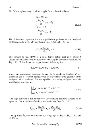
28                                                          Chapter 1
         The following boundary conditions apply for the fixed-free beam:


         The differential  equation for  the  equilibrium position  of  the  analyzed
         cantilever can be written by combining Eqs. (1.52) and (1.53) as:


          The solution  to Eq.  (1.90)  is a  third  degree polynomial in  x  whose 4
          unknown coefficients can be found by applying the boundary conditions of
          Eq. (1.89). This solution can be put into the following form:


          where the  distribution  functions  and  (b stands for bending, d for
          deflection and s for slope, respectively) are dependent on the geometry of the
          analyzed microcantilever. For  the  specific  case  being  analyzed  here, the
          distribution functions are:


          The slope  function is the derivative of the deflection function in terms of the
          space variable x, and therefore its equation derives from Eq. (1.91):


          The tip  force  can  be  expressed by  using  Eqs. (1.86),  (1.88),  (1.91) and
          (1.93) as: