Page 409 - Microsensors, MEMS and Smart Devices - Gardner Varadhan and Awadelkarim

APPLICATIONS 389

-0.0003 –0.00025 -0.0002 -0.00015 -0.0001 -0.00005
Distance from the edge of cavity (m)

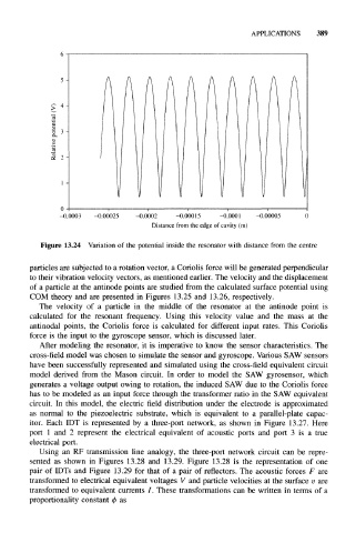
Figure 13.24 Variation of the potential inside the resonator with distance from the centre

particles are subjected to a rotation vector, a Coriolis force will be generated perpendicular
to their vibration velocity vectors, as mentioned earlier. The velocity and the displacement
of a particle at the antinode points are studied from the calculated surface potential using
COM theory and are presented in Figures 13.25 and 13.26, respectively.
The velocity of a particle in the middle of the resonator at the antinode point is
calculated for the resonant frequency. Using this velocity value and the mass at the
antinodal points, the Coriolis force is calculated for different input rates. This Coriolis
force is the input to the gyroscope sensor, which is discussed later.
After modeling the resonator, it is imperative to know the sensor characteristics. The
cross-field model was chosen to simulate the sensor and gyroscope. Various SAW sensors
have been successfully represented and simulated using the cross-field equivalent circuit
model derived from the Mason circuit. In order to model the SAW gyrosensor, which
generates a voltage output owing to rotation, the induced SAW due to the Coriolis force
has to be modeled as an input force through the transformer ratio in the SAW equivalent
circuit. In this model, the electric field distribution under the electrode is approximated
as normal to the piezoelectric substrate, which is equivalent to a parallel-plate capac-
itor. Each IDT is represented by a three-port network, as shown in Figure 13.27. Here
port 1 and 2 represent the electrical equivalent of acoustic ports and port 3 is a true
electrical port.
Using an RF transmission line analogy, the three-port network circuit can be repre-
sented as shown in Figures 13.28 and 13.29. Figure 13.28 is the representation of one
pair of IDTs and Figure 13.29 for that of a pair of reflectors. The acoustic forces F are
transformed to electrical equivalent voltages V and particle velocities at the surface v are
transformed to equivalent currents /. These transformations can be written in terms of a
proportionality constant 0 as