Page 199 - MODELING OF ASPHALT CONCRETE

VEPCD Modeling of Asphalt Concr ete with Gr owing Damage 177

Substituting this expression into Eq. (7-24), and rearranging and writing in the
discrete form, one finds the following equation:

⎛ (δ W ) ⎞ α (7-31)
R
t −
S = S + Δ ⎜ ⎝ d i ⎟ ⎠
i+1 i δ S
R
It must be observed that for the uniaxial case, the work function (W ) is given by
W = 1 C S()ε R (7-32)
R
2
Substituting Eq. (7-32) into (7-31) and simplifying, one arrives at
⎛ 1 (δ C ⎞ α
)
)
S = S + Δ t − (ε R 2 i ⎟ (7-33)
⎜
i+1 i ⎝ 2 δ S ⎠
In Eq. (7-33), it is assumed that before loading occurs, S and C are zero and one,
respectively. Further, dS must be specified and should be significantly less than the change
in damage over a time step (typically, 0.1 is used). After calculating the value of damage
(S) and the incremental damage (S + dS) at a given time step, the corresponding values of
i i
C are found by Eq. (7-29). The difference between these values (dC) is then used to calculate
damage at the next time step. The process is repeated until all data points are processed.
After completing this first iteration, the new values of S are plotted against the
original pseudostiffness values, and a new analytical relationship is found. The entire
process is repeated until the change in successive iterations is small. In this research,
eight such iterations were performed, but it was noted that very little improvement was
made after the third or fourth iteration.
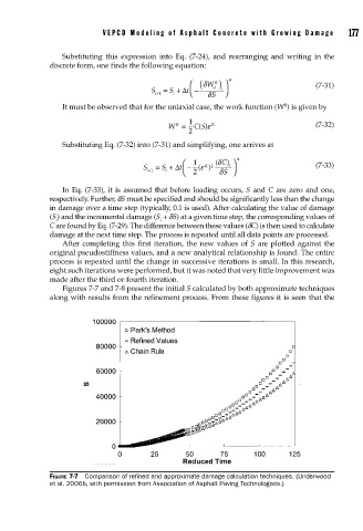
Figures 7-7 and 7-8 present the initial S calculated by both approximate techniques
along with results from the refinement process. From these figures it is seen that the

FIGURE 7-7 Comparison of refi ned and approximate damage calculation techniques. (Underwood
et al. 2006b, with permission from Association of Asphalt Paving Technologists.)