Page 208 - Modeling of Chemical Kinetics and Reactor Design

178 Modeling of Chemical Kinetics and Reactor Design

Table 3-6
t(sec) D 420 D – D
∞
0 0.120 0.661
900 0.290 0.491
1,800 0.420 0.361
2,700 0.510 0.271
3,600 0.581 0.200
4,500 0.632 0.149
∞ 0.781 0.0

that is,

D − D = ( D − D e – kt 1 (3-248)
)
∞
∞
O
Equation 3-248 is of the form
Y = Ae BX (3-249)

Linearizing Equation 3-249 gives

ln Y = ln A + BX (3-250)

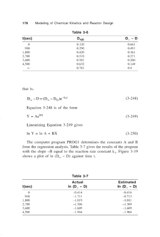
The computer program PROG1 determines the constants A and B
from the regression analysis. Table 3-7 gives the results of the program
with the slope –B equal to the reaction rate constant k . Figure 3-19
1
shows a plot of ln (D – D) against time t.
∞

Table 3-7
Actual Estimated
t(sec) ln (D – D) ln (D – D)
∞
∞
0 –0.414 –0.416
900 –1.711 –0.713
1,800 –1.019 –1.011
2,700 –1.306 –1.309
3,600 –1.609 –1.609
4,500 –1.904 –1.904