Page 128 - Modern Control Systems

102 Chapter 2 Mathematical Models of Systems

I
0.95

0.9

0.85
0.8 u
/ T" " " * " "'" T" " " " i
I i | -;_ j
- 0.75
I '
0.7
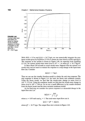
FIGURE 2.40 0.65
The tank water level
time history ob-
tained by integrat- 0.6 / !
ing the nonlinear
equations of motion 0.55 / ' j _ _ i
in Equation (2.125)
with H(0) = 0.5 m 0.5
and Q 1{f) = 0 50 100 150 200 250 300
Q* = 34.77 kg/s. Time (s)

With //(0) = 0.5 m and Q\{t) = 34.77 kg/s, we can numerically integrate the non-
linear model given by Equation (2.125) to obtain the time history of H(t) and £^(0-
The response of the system is shown in Figure 2.40. As expected from Equation
3
(2.114), the system steady-state water level is H* = 1 m when Q* = 34.77 kg/m .
It takes about 250 seconds to reach steady-state. Suppose that the system is at
steady state and we want to evaluate the response to a step change in the input mass
flow rate. Consider
AQi(0 = 1 kg/s.

Then we can use the transfer function model to obtain the unit step response. The
step response is shown in Figure 2.41 for both the linear and nonlinear models.
Using the linear model, we find that the steady-state change in water level is
AH = 5.75 cm. Using the nonlinear model, we find that the steady-state change in
water level is AH = 5.84 cm. So we see a small difference in the results obtained
from the linear model and the more accurate nonlinear model.
As the final step, we consider the system response to a sinusoidal change in the
input flow rate. Let

AQiO?) = 2 ^ 2,
s + or
where &> = 0.05 rad/s and q a = 1. The total water input flow rate is
Q x(t) = Q* + AQ x(t),

where Q* = 34.77 kg/s. The output flow rate is shown in Figure 2.42.