Page 125 - Modern Control Systems

Section 2.8 Design Examples 99

and
dh
= 0.
3(2i
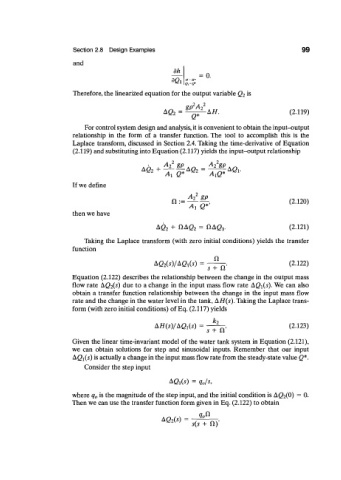
Therefore, the linearized equation for the output variable Q 2 is

A<2 2 = ^ ^ A / / - ( 2 1 1 9 )

For control system design and analysis, it is convenient to obtain the input-output
relationship in the form of a transfer function. The tool to accomplish this is the
Laplace transform, discussed in Section 2.4. Taking the time-derivative of Equation
(2.119) and substituting into Equation (2.117) yields the input-output relationship

2
A 2
A/S . 2 8P Kri A 2 gp ^
A
A G 2 + A ( ? 2 = A G l
^ ^ ^ -
If we define
0 : = ^ ^ , (2.120)
then we have

AQ 2 + flAQ 2 = OAQi. (2.121)
Taking the Laplace transform (with zero initial conditions) yields the transfer
function

AQ 2(s)/AQ l(s) = - £ - . (2.122)
s + 12
Equation (2.122) describes the relationship between the change in the output mass
flow rate AQ 2{s) due to a change in the input mass flow rate AQ x(s). We can also
obtain a transfer function relationship between the change in the input mass flow
rate and the change in the water level in the tank, AH(s). Taking the Laplace trans-
form (with zero initial conditions) of Eq. (2.117) yields

AHisyAQds) = j ^ . (2.123)
Given the linear time-invariant model of the water tank system in Equation (2.121),
we can obtain solutions for step and sinusoidal inputs. Remember that our input
AQi(s) is actually a change in the input mass flow rate from the steady-state value Q*.
Consider the step input

AQiCs) = q 0/s,

where q 0 is the magnitude of the step input, and the initial condition is AQ 2{0) = 0.
Then we can use the transfer function form given in Eq. (2.122) to obtain

AQ2(S) =
Krnry