Page 122 - Modern Control Systems

Chapter 2 Mathematical Models of Systems

the reservoir and output pipe. We can neglect viscosity in our model development.
We say our fluid is inviscid.
If each fluid element at each point in the flow has no net angular velocity about
that point, the flow is termed irrotational. Imagine a small paddle wheel immersed
in the fluid (say in the output port). If the paddle wheel translates without rotating,
the flow is irrotational. We will assume the water in the tank is irrotational. For an
inviscid fluid, an initially irrotational flow remains irrotational.
The water flow in the tank and output port can be either steady or unsteady. The
flow is steady if the velocity at each point is constant in time. This does not neces-
sarily imply that the velocity is the same at every point but rather that at any given
point the velocity does not change with time. Steady-state conditions can be
achieved at low fluid speeds. We will assume steady flow conditions. If the output
port area is too large, then the flow through the reservoir may not be slow enough to
establish the steady-state condition that we are assuming exists and our model will
not accurately predict the fluid flow motion.
To obtain a mathematical model of the flow within the reservoir, we employ
basic principles of science and engineering, such as the principle of conservation of
mass. The mass of water in the tank at any given time is

m = A XH, (2.108)
P
where A x is the area of the tank, p is the water density, and H is the height of the
water in the reservoir. The constants for the reservoir system are given in Table 2.7.
In the following formulas, a subscript 1 denotes quantities at the input, and a
subscript 2 refers to quantities at the output. Taking the time derivative of m in
Equation (2.108) yields
m = pA^H,
where we have used the fact that our fluid is incompressible (that is, p = 0) and that
the area of the tank, A h does not change with time. The change in mass in the reser-
voir is equal to the mass that enters the tank minus the mass that leaves the tank, or

m = pA xH = Qi- pA 2v 2, (2.109)
where £?i is the steady-state input mass flow rate, v 2 is the exit velocity, and A 2 is the
output port area. The exit velocity, v 2, is a function of the water height. From
Bernoulli's equation [39] we have

2
-pvf+ A + pgH = -pv 2 + P 2,
where Vi is the water velocity at the mouth of the reservoir, and Pi and P 2 are the at-
and P 2 are equal to
mospheric pressures at the input and output, respectively. But P x

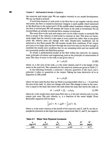
Table 2.7 Water Tank Physical Constants
P g A 1 A 2 H* Q*
3 2 2 2
(kg/m ) (m/s ) [m ] [m ] (m) (kg/s)
1000 9.8 TT/4 IT/400 1 34.77