Page 120 - Modern Control Systems

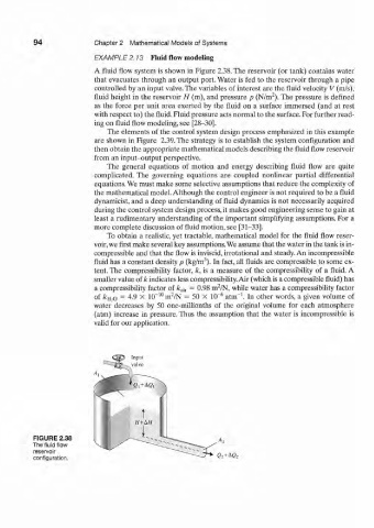
94 Chapter 2 Mathematical Models of Systems

EXAMPLE 2.13 Fluid flow modeling
A fluid flow system is shown in Figure 2.38. The reservoir (or tank) contains water
that evacuates through an output port. Water is fed to the reservoir through a pipe
controlled by an input valve. The variables of interest are the fluid velocity V (m/s),
2
fluid height in the reservoir H (m), and pressure p (N/m ). The pressure is defined
as the force per unit area exerted by the fluid on a surface immersed (and at rest
with respect to) the fluid. Fluid pressure acts normal to the surface. For further read-
ing on fluid flow modeling, see [28-30],
The elements of the control system design process emphasized in this example
are shown in Figure 2.39. The strategy is to establish the system configuration and
then obtain the appropriate mathematical models describing the fluid flow reservoir
from an input-output perspective.
The general equations of motion and energy describing fluid flow are quite
complicated. The governing equations are coupled nonlinear partial differential
equations. We must make some selective assumptions that reduce the complexity of
the mathematical model. Although the control engineer is not required to be a fluid
dynamicist, and a deep understanding of fluid dynamics is not necessarily acquired
during the control system design process, it makes good engineering sense to gain at
least a rudimentary understanding of the important simplifying assumptions. For a
more complete discussion of fluid motion, see [31-33].
To obtain a realistic, yet tractable, mathematical model for the fluid flow reser-
voir, we first make several key assumptions. We assume that the water in the tank is in-
compressible and that the flow is inviscid, irrotational and steady. An incompressible
3
fluid has a constant density p (kg/m ). In fact, all fluids are compressible to some ex-
tent. The compressibility factor, k, is a measure of the compressibility of a fluid. A
smaller value of k indicates less compressibility. Air (which is a compressible fluid) has
2
a compressibility factor of k. Ail = 0.98 m /N, while water has a compressibility factor
o f -10 2 6 1
^H 2O = 4.9 x 10 m /N = 50 x 10~ atnT . In other words, a given volume of
water decreases by 50 one-millionths of the original volume for each atmosphere
(atm) increase in pressure. Thus the assumption that the water is incompressible is
valid for our application.

Input
valve

FIGURE 2.38
The fluid flow
reservoir
configuration.