Page 115 - Modern Control Systems

Section 2.7 Signal-Flow Graph Models 89

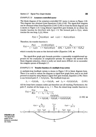
EXAMPLE 2.9 Armature-controlled motor
The block diagram of the armature-controlled DC motor is shown in Figure 2.20.
This diagram was obtained from Equations (2.64)-(2.68). The signal-flow diagram
can be obtained either from Equations (2.64)-(2.68) or from the block diagram and
is shown in Figure 2.32. Using Mason's signal-flow gain formula, let us obtain the
transfer function for 6(s)/V a(s) with T d(s) - 0. The forward path is P\(s), which
touches the one loop, Li(s), where

PI(J) - - j G ^ G ^ ) and L }(s) =-K hG 1(s)G 2(s).

Therefore, the transfer function is

P l(s) (l/s)G,(s)G 2(s) K„
T(s) =
1 - Us) 1 + K hG l(s)G 2(s) s[(R a + L as)(Js + b) + K bK m\
which is exactly the same as that derived earlier (Equation 2.69). •

The signal-flow graph gain formula provides a reasonably straightforward ap-
proach for the evaluation of complicated systems. To compare the method with
block diagram reduction, which is really not much more difficult, let us reconsider
the complex system of Example 2.7.
EXAMPLE 2.10 Transfer function of a multiple-loop system

A multiple-loop feedback system is shown in Figure 2.26 in block diagram form.
There is no need to redraw the diagram in signal-flow graph form, and so we shall
proceed as usual by using Mason's signal-flow gain formula, Equation (2.98). There
is one forward path P : = G1G2G2G4. The feedback loops are

L x = -G 2G 3H 2, L 2 = G 2G 4H l, and L 3 = -GfoG&fy. (2.101)
All the loops have common nodes and therefore are all touching. Furthermore, the
path Pj touches all the loops, so Aj = 1. Thus, the closed-loop transfer function is
Y(s) Pi A
1^1
T(s) =
R(s) 1 L\ — L 2 — LT,
G]G 2G-3 )Gi l
(2.102)
1 + G 2G^H 2 — G2G4H1 + 0^02^3(.74./73

W O O »<*>
FIGURE 2.32
The signal-flow
graph of the
armature-controlled
DC motor.