Page 111 - Modern Control Systems

Section 2.7 Signal-Flow Graph Models 85
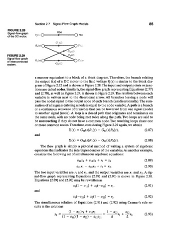
FIGURE 2.28
Signal-flow graph G(s)
of the DC motor. VfMQ- — • — -O <*s)

G u{s)
R,(s) YAs)

FIGURE 2.29
Signal-flow graph
of interconnected Rils) y-.ro
system. G 22(s)

a manner equivalent to a block of a block diagram. Therefore, the branch relating
the output 6{s) of a DC motor to the field voltage Vf{s) is similar to the block dia-
gram of Figure 2.22 and is shown in Figure 2.28. The input and output points or junc-
tions are called nodes. Similarly, the signal-flow graph representing Equations (2.77)
and (2.78), as well as Figure 2.24, is shown in Figure 2.29. The relation between each
variable is written next to the directional arrow. All branches leaving a node will
pass the nodal signal to the output node of each branch (unidirectionally).The sum-
mation of all signals entering a node is equal to the node variable. A path is a branch
or a continuous sequence of branches that can be traversed from one signal (node)
to another signal (node). A loop is a closed path that originates and terminates on
the same node, with no node being met twice along the path. Two loops are said to
be nontouching if they do not have a common node. Two touching loops share one
or more common nodes. Therefore, considering Figure 2.29 again, we obtain
Y x(s) = GuWR^s) + G 12(s)R 2(s), (2.87)
and
Y 2(s) = G 2l(s)R 1(s) + G 22(s)R 2(s). (2.88)
The flow graph is simply a pictorial method of writing a system of algebraic
equations that indicates the interdependencies of the variables. As another example,
consider the following set of simultaneous algebraic equations:
a r x
ii*i + #12*2 + \ — \ (2.89)
«21*1 + «22*2 + r 2 = x 2. (2.90)
The two input variables are r\ and r 2, and the output variables are X\ and x 2. A sig-
nal-flow graph representing Equations (2.89) and (2.90) is shown in Figure 2.30.
Equations (2.89) and (2.90) may be rewritten as
*i(l - «n) + *2(-«i2> = r h (2.91)
and
*i(-«2i) + x 2(l - «22) = r 2. (2.92)
The simultaneous solution of Equations (2.91) and (2.92) using Cramer's rule re-
sults in the solutions
(1 - 022)'! + «12?2 1 ~ «22 , «12 / 0 ^ ,
Xi =
T
(1 - «ll)(l ~ «22) ~ «12-21 —£—r, + , 2 , (2.93)