Page 106 - Modern Control Systems

80 Chapter 2 Mathematical Models of Systems

FIGURE 2.22 V f(s). Output
Block diagram of a G(s) = s(Js + b)(L fs + R f) • 0U)
DC motor.
FIGURE 2.23
General block
representation of
two-input, two-
output system.

the input and output variables. Therefore, one can correctly assume that the transfer
function is an important relation for control engineering.
The importance of this cause-and-effect relationship is evidenced by the facility
to represent the relationship of system variables by diagrammatic means. The block
diagram representation of the system relationships is prevalent in control system en-
gineering. Block diagrams consist of unidirectional, operational blocks that represent
the transfer function of the variables of interest. A block diagram of a field-con-
trolled DC motor and load is shown in Figure 2.22. The relationship between the dis-
placement 8(s) and the input voltage Vf(s) is clearly portrayed by the block diagram.
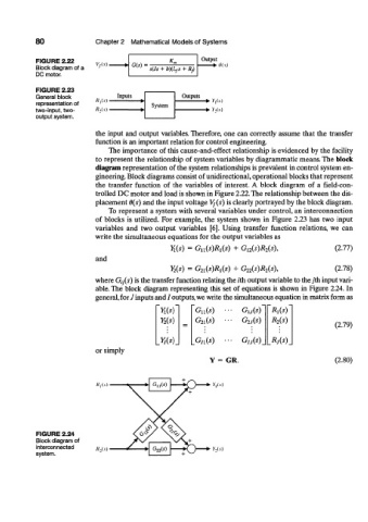
To represent a system with several variables under control, an interconnection
of blocks is utilized. For example, the system shown in Figure 2.23 has two input
variables and two output variables [6]. Using transfer function relations, we can
write the simultaneous equations for the output variables as
Yi(s) = G n(s)R 1(s) + G l2(s)R 2(s), (2.77)
and
Y 2(s) = GhWRAs) + G 22(s)R 2(s), (2.78)
where G^s) is the transfer function relating the ith output variable to theyth input vari-
able. The block diagram representing this set of equations is shown in Figure 2.24. In
general, for J inputs and I outputs, we write the simultaneous equation in matrix form as

Yi(s) G n(s) ••• G v(s) R^s)
Y 2(s) G 21(s) ••• G 2J(s) R 2(s)
(2.79)

Ji(s). _G n(s) ••• Gjj(s)_ _Rj(s)_
or simply
Y = GR. (2.80)

RA\) G n(s) — • n — • K,(.Y)

FIGURE 2.24
Block diagram of
interconnected R,(s) YM.s)
system.