Page 108 - Modern Control Systems

82 Chapter 2 Mathematical Models of Systems

Controller Actuator Process
E a(s) Z{s) Uis)
O
/?(.v) G c(s) G a(s) G(s) •+> n.s)

Sensor
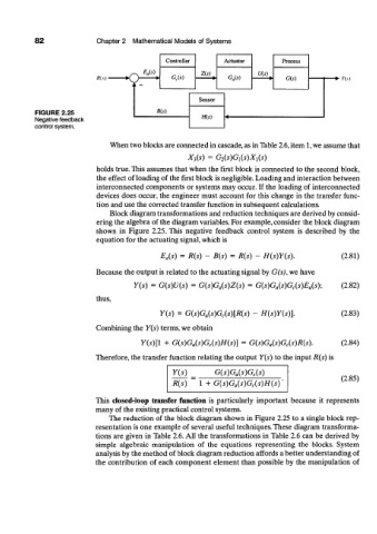
FIGURE 2.25 B(s)
Negative feedback H{s)
control system.

When two blocks are connected in cascade, as in Table 2.6, item 1, we assume that
X 3(s) = G 2(s)G 1(s)X 1(s)
holds true. This assumes that when the first block is connected to the second block,
the effect of loading of the first block is negligible. Loading and interaction between
interconnected components or systems may occur. If the loading of interconnected
devices does occur, the engineer must account for this change in the transfer func-
tion and use the corrected transfer function in subsequent calculations.
Block diagram transformations and reduction techniques are derived by consid-
ering the algebra of the diagram variables. For example, consider the block diagram
shown in Figure 2.25. This negative feedback control system is described by the
equation for the actuating signal, which is

E a(s) = R(s) - B(s) = R(s) - H(s)Y(s). (2.81)

Because the output is related to the actuating signal by G(s), we have
Y(s) = G(s)U(s) = G(s)G a(s)Z(s) = G(s)G a(s)G c(s)E a(s); (2.82)
thus,

Y(s) = G(s)G a(s)G c(s)[R(s) - H(s)Y(s)]. (2.83)
Combining the Y(s) terms, we obtain

Y(s)[l + G(s)G a(s)G c(s)H(s)] = G(s)G a(s)G c(s)R(s). (2.84)
Therefore, the transfer function relating the output Y(s) to the input R(s) is

Y(s) = G(s)G a(s)G c(s)
(2.85)
R(s) 1 + G(s)G a(s)G c(s)H(s)'

This closed-loop transfer function is particularly important because it represents
many of the existing practical control systems.
The reduction of the block diagram shown in Figure 2.25 to a single block rep-
resentation is one example of several useful techniques. These diagram transforma-
tions are given in Table 2.6. All the transformations in Table 2.6 can be derived by
simple algebraic manipulation of the equations representing the blocks. System
analysis by the method of block diagram reduction affords a better understanding of
the contribution of each component element than possible by the manipulation of