Page 130 - Modern Control Systems

104 Chapter 2 Mathematical Models of Systems

1.04

1.03

1.02

1.01

0.99

0.98
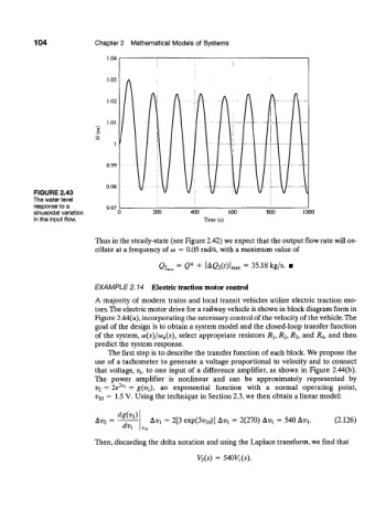
FIGURE 2.43
The water level
response to a 0.97
sinusoidal variation 200 400 600 800 1000
in the input flow. Time (s)

Thus in the steady-state (see Figure 2.42) we expect that the output flow rate will os-
cillate at a frequency of at — 0.05 rad/s, with a maximum value of

Qo =Q* + |AQ 2(0l max = 35.18 kg/s. •

EXAMPLE 2.14 Electric traction motor control
A majority of modern trains and local transit vehicles utilize electric traction mo-
tors. The electric motor drive for a railway vehicle is shown in block diagram form in
Figure 2.44(a), incorporating the necessary control of the velocity of the vehicle. The
goal of the design is to obtain a system model and the closed-loop transfer function
of the system, a)(s)/a) d(s), select appropriate resistors R h R 2, R$, and R A, and then
predict the system response.
The first step is to describe the transfer function of each block. We propose the
use of a tachometer to generate a voltage proportional to velocity and to connect
that voltage, v u to one input of a difference amplifier, as shown in Figure 2.44(b).
The power amplifier is nonlinear and can be approximately represented by
2vx
v 2 = 2e = g(vi), an exponential function with a normal operating point,
v w = 1.5 V. Using the technique in Section 2.3, we then obtain a linear model:

dgM
Ai>> = Av y = 2[3 exp(3w 10)] A^ = 2(270) A^ = 540 A^. (2.126)
dvi
«10
Then, discarding the delta notation and using the Laplace transform, we find that

V 2(s) = StoV^s).