Page 156 - Modern Control Systems

130 Chapter 2 Mathematical Models of Systems

0.12

0.1
/' i
0.08
—, /__ + 1 ,
i / i
0.06
I / : i
0.04 /j __. [
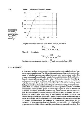
FIGURE 2.78 / i
The system 0.02
response of the
system shown in
Figure 2.77 for 0
0 0.1 0.2 0.3 0.4 0.5 0.6 0.7
R(s) = — .
Time (s)

Using the approximate second-order model for G(s), we obtain

Y(s) 5K n
R(s) s 1 + 20s + 5K a
When Ka = 40, we have
200
Y(s) 2 R(s).
s + 20s + 200
0.1
We obtain the step response for R(s) — — rad, as shown in Figure 2.78.

2.11 SUMMARY
In this chapter, we have been concerned with quantitative mathematical models of con-
trol components and systems. The differential equations describing the dynamic perfor-
mance of physical systems were utilized to construct a mathematical model. The
physical systems under consideration included mechanical, electrical, fluid, and thermo-
dynamic systems. A linear approximation using a Taylor series expansion about the op-
erating point was utilized to obtain a small-signal linear approximation for nonlinear
control components. Then, with the approximation of a linear system, one may utilize
the Laplace transformation and its related input-output relationship given by the trans-
fer function. The transfer function approach to linear systems allows the analyst to
determine the response of the system to various input signals in terms of the location
of the poles and zeros of the transfer function. Using transfer function notations, block dia-
gram models of systems of interconnected components were developed. The block
relationships were obtained. Additionally, an alternative use of transfer function models
in signal-flow graph form was investigated. Mason's signal-flow gain formula was inves-
tigated and was found to be useful for obtaining the relationship between system variables
in a complex feedback system. The advantage of the signal-flow graph method was the
availability of Mason's signal-flow gain formula, which provides the relationship
between system variables without requiring any reduction or manipulation of the flow