Page 152 - Modern Control Systems

126 Chapter 2 Mathematical Models of Systems

No common factors Possible common factors
T(s) = sys G(s) ~ sysl

FIGURE 2.70
The minreal sys=r Tiinr< 3al(sys1)
function.

»num=[1 4 6 6 5 21; den=[12 205 1066 2517 3128 2196 712];
»sys1 =tf(num,den);
»sys=minreal(sys1); M Cancel common factors.
Transfer function:
FIGURE 2.71 0.08333 sM + 0.25 s 3 + 0.25 s 2 + 0.25 s + 0.1667
A
A
Application of the A A A
s 5 + 16.08 sM + 72.75 s 3 + 137 s 2 + 123.7 s + 59.33
minreal function.
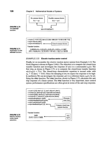
EXAMPLE 2.23 Electric traction motor control

Finally, let us reconsider the electric traction motor system from Example 2.14. The
block diagram is shown in Figure 2.44(c). The objective is to compute the closed-loop
transfer function and investigate the response of <o(s) to a commanded Q)d(s). The
first step, as shown in Figure 2.72, is to compute the closed-loop transfer function
a)(s)/(o d(s) = T(s). The closed-loop characteristic equation is second order with
(o n = 52 and £ = 0.012. Since the damping is low, we expect the response to be high-
ly oscillatory. We can investigate the response <o(t) to a reference input, <o d(t), by uti-
lizing the step function. The step function, shown in Figure 2.73, calculates the unit
step response of a linear system. The step function is very important, since control
system performance specifications are often given in terms of the unit step response.

»num1=["IO]; den1=[1 1]; sys1=tf(num1,den1);
»num2=[1]; den2=[2 0.5]; sys2=tf{num2,den2);
»num3=[540]; den3=[1]; sys3=tf(num3,den3);
»num4-[0.1]; den4-[1]; sys4-tf(num4,den4);
»svs5=series(svs1 ,svs2); Eliminate
»sys6=feedback{sys5,sys4); " inner loop
»sys7=series(sys3,sys6);
»sys=feedback(sys7,[1]) M 1
Compute closed-loop
transfer function

Transfer function:
FIGURE 2.72 5400 w(s)
Electric traction A
motor block 2 s 2 + 2.5 s + 5402 ' <o d(s)
reduction.