Page 147 - Modern Control Systems

Section 2.9 The Simulation of Systems Using Control Design Software 121

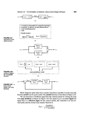
s+ 1 U(s)
/Us) G,(i) G(s) = z Yis)
s + 2 500 «
(a)

»numg=[1]; deng=[500 0 0]; sysg=tf(numg,deng);
»numh=[1 1]; denh=[1 2]; sysh=tf(numh,denh);
»sys=series(sysg,sysh);
»sys
Transfer function:
s + 1
G c(s)G(s)
A
A
500 s 3 +1000 s 2
FIGURE 2.61
Application of the
series function. (b)
System 1
C,(5)
Uis - • Y(s)
System 2
G 2(s)

(a)

T(s) = =sys G]Cs) = sysl G 2(s) = sys2
W)
t ,
]=P arallel(sy 1
1 1
FIGURE 2.62
(a) Block diagram. [sys s1,sys2)
(b) The parallel
function. (b)

W Controller U(.s) Process
R(s) ^ O • • Y(.\
G c(s) G(s)
FIGURE 2.63 A
basic control
system with unity
feedback.

Block diagrams quite often have transfer functions in parallel. In such cases, the
function parallel can be quite useful. The parallel function is described in Figure 2.62.
We can introduce a feedback signal into the control system by closing the loop
with unity feedback, as shown in Figure 2.63. The signal E a(s) is an error signal; the
signal R(s) is a reference input. In this control system, the controller is in the for-
ward path, and the closed-loop transfer function is

G c(s)G(s)
T(s) =
1 =F G c(s)G(s)'