Page 145 - Modern Control Systems

Section 2.9 The Simulation of Systems Using Control Design Software 119

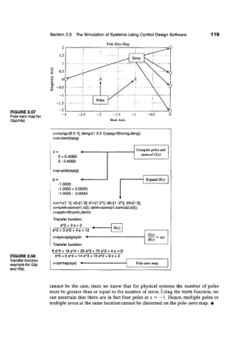
Pole-Zero Map

FIGURE 2.57
Pole-zero map for
G(s)/H(s).

»numg=[6 0 1]; deng=[1 3 3 1];sysg=tf(numg,deng);
»z=zero(sysg)

Compute poles and
Z- -4-
zeros of G(s)
0 + 0.4082i
0 - 0.4082J
»p=pole(sysg)

P = Expand H(s)
-1.0000
-1.0000 + O.OOOOi
-1.0000- O.OOOOi
'
»n1=[1 1]; n2=[1 2]; d1=[1 2*i]; d2=[1 -2*i]; d3=[1 3];
»numh=conv(n1,n2); denh=conv(d1 ,conv(d2,d3));
»sysh=tf(numh,denh)
Transfer function:
A
s 2 + 3 s + 2
fi{s)
A
A
4
s 3 + 3s 2 + s + 12
G(s)
»sys=sysg/sysh -*— = sys
H(s)
Transfer function:
A
A
A
6 s 5 +18 sM + 25 s 3 + 75 s 2 + 4 s +12
A
A
A
FIGURE 2.58 s 5 + 6 sM + 14 s 3 + 16 s 2 + 9 s + 2
Transfer function
example for G{s) »pzmap(sys) ^ Pole-zero map
and H(s).
cannot be the case, since we know that for physical systems the number of poles
must be greater than or equal to the number of zeros. Using the roots function, we
can ascertain that there are in fact four poles at s = —1. Hence, multiple poles or
multiple zeros at the same location cannot be discerned on the pole-zero map. •