Page 150 - Modern Control Systems

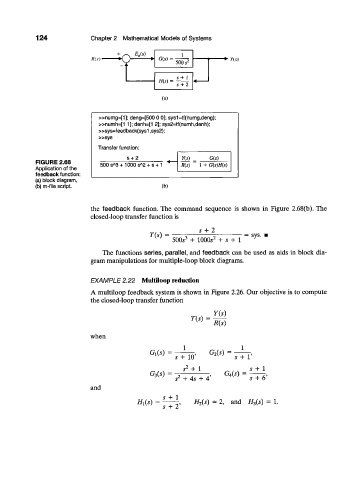
124 Chapter 2 Mathematical Models of Systems

+ - . E a{s)
Ris) • o G(s) = 500 s 2 - • Y(s)

s + I
H{s) =
s + 2
(a)

»numg=[1]; deng=[500 0 0]; sys1=tf(numg,deng);
»numh=[1 1];denh=[1 2]; sys2=tf(numh,denh);
»sys=feedback(sys1 ,sys2);
»sys
Transfer function:
s + 2 Y(s) Gis)
FIGURE 2.68 500 s*3 + 1000 s 2 + s + 1 * R(s) 1 + G(s)H(s)
A
Application of the
feedback function:
(a) block diagram,
(b) m-file script. (b)

the feedback function. The command sequence is shown in Figure 2.68(b). The
closed-loop transfer function is
s + 2
T(s) = 3 2 = sys.
500s + 1000^ + 5 + 1

The functions series, parallel, and feedback can be used as aids in block dia-
gram manipulations for multiple-loop block diagrams.

EXAMPLE 2.22 Multiloop reduction
A multiloop feedback system is shown in Figure 2.26. Our objective is to compute
the closed-loop transfer function

Y(s)
T{s) =
R(s)

when
1 1
G 1(s) = G 2(s) =
s + 10' 5 + V
s 2 + 1 5 + 1
G 3(s) = 2 G 4(s) =
5 + 45 + 4' 5 + 6'
and
5 + 1
H^s) = H 2(s) = 2, and //3(5) = 1.
5 + 2'