Page 148 - Modern Control Systems

122 Chapter 2 Mathematical Models of Systems

System 1
R(s) • • Y(s)
G c(s)G(s)

(a)

+1 - positive feedback
T(s) = =sys G c{s)G{s) = sysl
Ks) — 1 - negative feedback (default)
i r
FIGURE 2.64
(a) Block diagram. [sys]=feedback(sys1 ,[1],sign)
(b) The feedback
function with unity
feedback. (b)

R(s) • Q ». System 1 -*- Y(s)
G(s)

System 2
His)
(a)

s
r ( ) = = s G(s) = sysl H(s) = sys2 +1 - pos. feedback
* i | y - 1 - neg. feedback
(default)
i i
i \. 1 i
FIGURE 2.65 [sysj=feedback(sy s1,sys2 .sign)
(a) Block diagram.
(b) The feedback
function. (b)

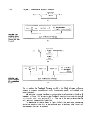
We can utilize the feedback function to aid in the block diagram reduction
process to compute closed-loop transfer functions for single- and multiple-loop
control systems.
It is often the case that the closed-loop control system has unity feedback, as il-
lustrated in Figure 2.63. We can use the feedback function to compute the closed-
loop transfer function by setting H(s) = 1. The use of the feedback function for
unity feedback is depicted in Figure 2.64.
The feedback function is shown in Figure 2.65 with the associated system con-
figuration, which includes H(s) in the feedback path. If the input "sign" is omitted,
then negative feedback is assumed.