Page 143 - Modern Control Systems

Section 2.9 The Simulation of Systems Using Control Design Software 1 1 7

» num1=[10];den1=[1 2 5];
» sys1=tf(num1,den1)

Transfer function:
I
10
Transfer function G(s) = _ num 4 GAs)
A
i object "ST s 2 + 2 s + 5
I I » » num2=[1];den2=[1 1];
sys2=tf(num2,den2)
sys = tf(num,den)
Transfer function:
1
G 2(s)
s + 1
»sys=sys1+sys2
FIGURE 2.54
(a) The tf function. Transfer function:
(b) Using the tf s 2 + 12s+15
A
function to create Giis) + G 2(s)
transfer function A A
objects and adding s 3 + 3 s 2 + 7 s + 5
t
them using he"+"
operator. (a) (b)
The function polyval is used to evaluate the value of a polynomial at the given
value of the variable. The polynomial n(s) has the value n(—5) = -66, as shown in
Figure 2.53.
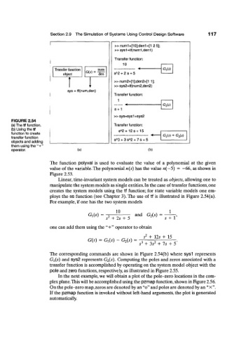
Linear, time-invariant system models can be treated as objects, allowing one to
manipulate the system models as single entities. In the case of transfer functions, one
creates the system models using the tf function; for state variable models one em-
ploys the ss function (see Chapter 3). The use of tf is illustrated in Figure 2.54(a).
For example, if one has the two system models

10 1
G,(s) = 2 and G 2(s) =
s + 2s + 5 s + V
one can add them using the "+" operator to obtain

s 2 + 12s + 15
G(s) = G,(s) ~ G 2(s) = 3 2
s + 3s + 7s + 5
The corresponding commands are shown in Figure 2.54(b) where sysl represents
Gi(s) and sys2 represents G^Cs). Computing the poles and zeros associated with a
transfer function is accomplished by operating on the system model object with the
pole and zero functions, respectively, as illustrated in Figure 2.55.
In the next example, we will obtain a plot of the pole-zero locations in the com-
plex plane. This will be accomplished using the pzmap function, shown in Figure 2.56.
On the pole-zero map, zeros are denoted by an "o" and poles are denoted by an "X".
If the pzmap function is invoked without left-hand arguments, the plot is generated
automatically.