Page 146 - Modern Control Systems

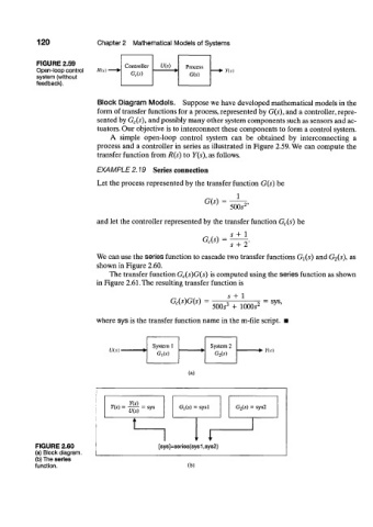
120 Chapter 2 Mathematical Models of Systems

FIGURE 2.59 Controller
Open-loop control fUs) tt.v)
system (without C,(s)
feedback).

Block Diagram Models. Suppose we have developed mathematical models in the
form of transfer functions for a process, represented by G(s), and a controller, repre-
sented by G c(s), and possibly many other system components such as sensors and ac-
tuators. Our objective is to interconnect these components to form a control system.
A simple open-loop control system can be obtained by interconnecting a
process and a controller in series as illustrated in Figure 2.59. We can compute the
transfer function from R(s) to Y(s), as follows.

EXAMPLE 2.19 Series connection
Let the process represented by the transfer function G(s) be

G(s) = —?-r,
v 2
500^
and let the controller represented by the transfer function G c(s) be
s + 1
G c(s) =
5 + 2'
We can use the series function to cascade two transfer functions G\(s) and G 2(s), as
shown in Figure 2.60.
The transfer function G c(s)G(s) is computed using the series function as shown
in Figure 2.61 .The resulting transfer function is

5 + 1
G c(s)G(s) = 3 2 SyS
500^ + 1000^ ~ '
where sys is the transfer function name in the m-file script.

** Y(s)

(a)

7Y ^ ^ ) G,(*) = sysl G 2(s) = sys2

i L
1
[si /s]= :series(sy I I
FIGURE 2.60
(a) Block diagram.
(b) The series s1 ,sys2)
function. (b)