Page 151 - Modern Control Systems

Section 2.9 The Simulation of Systems Using Control Design Software 125

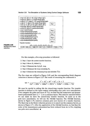
»ng1=[1]; dg1=[1 10]; sysg1=tf(ng1,dg1);
»ng2=[1]; dg2=[1 1]; sysg2=tf(ng2,dg2);
»ng3=[1 0 1]; dg3=[1 4 4]; sysg3=tf(ng3,dg3);
»ng4={1 1]; dg4=[1 6]; sysg4=tf(ng4,dg4);
»nh1=[1 1];dh1=[1 2]; sysh1=tf(nh1,dh1); Step 1
»nh2=[2]; dh2=[1]; sysh2=tf(nh2,dh2);
»nh3=[1]; dh3=[1]; sysh3=tf(nh3,dh3);
»sys 1 =sysh2/sysg4; Step 2
»sys2=series(sysg3,sysg4);
»sys3=feedback(sys2,sysh1 ,+1); Step 3
»sys4=series(sysg2,sys3);
»sys5=feedback(sys4,sys1);
Step 4
»sys6=series(sysg1 ,sys5);
»sys=feedback(sys6,sysh3);
Step 5
Transfer function:
FIGURE 2.69 s 5 + 4 sM + 6 s 3 + 6 s 2 + 5 s + 2
A
A
A
Multiple-loop block 12 s ^ + 205 s 5 + 1066 sM + 2517 s 3 + 3128 s 2 + 2196 s + 712
A
A
A
reduction.
For this example, a five-step procedure is followed:

Q Step 1. Input the system transfer functions.
• Step 2. Move H 2 behind G 4 .
~) Step 3. Eliminate the G 3G^Hi loop.
0 Step 4. Eliminate the loop containing H 2.
• Step 5. Eliminate the remaining loop and calculate T(s).
The five steps are utilized in Figure 2.69, and the corresponding block diagram
reduction is shown in Figure 2.27. The result of executing the commands is
A
s 5 + As + 6s 3 + 6s 2 + 5s + 2
sys = 6 5 4 3 2
12s + 205s + 10665 + 2517s + 3128s + 2196s + 712'

We must be careful in calling this the closed-loop transfer function. The transfer
function is defined as the input-output relationship after pole-zero cancellations.
If we compute the poles and zeros of T(s), we find that the numerator and denom-
inator polynomials have (s + 1) as a common factor. This must be canceled before
we can claim we have the closed-loop transfer function. To assist us in the
pole-zero cancellation, we will use the minreal function. The minreal function,
shown in Figure 2.70, removes common pole-zero factors of a transfer function.
The final step in the block reduction process is to cancel out the common factors, as
shown in Figure 2.71. After the application of the minreal function, we find that the
order of the denominator polynomial has been reduced from six to five, implying
one pole-zero cancellation. •