Page 144 - Modern Control Systems

118 Chapter 2 Mathematical Models of Systems

»sys=tf([1 101J1 2 1])

Transfer function:
s + 10
Poles
A
s 2 + 2 s + 1
sys
p=pole(sys)
Transfer
function
object P=
z=zero(sys)
•1 -
•1
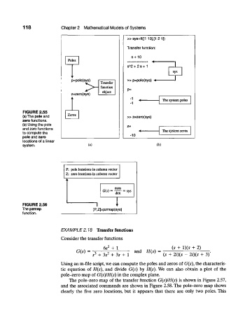
FIGURE 2.55
Zeros
(a) The pole and » z=zero(sys)
zero functions.
(b) Using the pole z=
and zero functions
to compute the The system zeros
pole and zero -10
locations of a linear
system. (a) (b)

P: pole locations in column vector
Z: zero locations in column vector

G(s)
= 1 ^ = ^

FIGURE 2.56
The pzmap [P,Z]=pzmap(sys)
function.

EXAMPLE 2.18 Transfer functions
Consider the transfer functions

6s 2 + 1 (s + 1)(5 + 2)
G(s) = 3 2 and H(s) =
5 + 3s + 3s + 1 (s + 2/)(5 - 2i)(s + 3)'
Using an m-file script, we can compute the poles and zeros of G(s), the characteris-
tic equation of H(s), and divide G(s) by H(s). We can also obtain a plot of the
pole-zero map of G(s)IH(s) in the complex plane.
The pole-zero map of the transfer function G(s)IH(s) is shown in Figure 2.57,
and the associated commands are shown in Figure 2.58. The pole-zero map shows
clearly the five zero locations, but it appears that there are only two poles. This