Page 141 - Modern Control Systems

Section 2.9 The Simulation of Systems Using Control Design Software 115

»y0=0.15;
»wn=sqrt(2); <
»zeta=1/(2*sqrt(2));
»t=[0:0.1:10];
»unforced
unforced.m
%Compute Unforced Response to an Initial Condition
%
A
c=(yO/sqrt(1-zeta 2)); ««- y(0)/Vl - p
A
y=c*exp(-zeta*wn*t) .*sin(wn*sqrt(1 -zeta 2)*t+acos(zeta));
%
bu=c*exp(-zeta*wn*t);bl=-bu; -* e &"' envelope
%
,
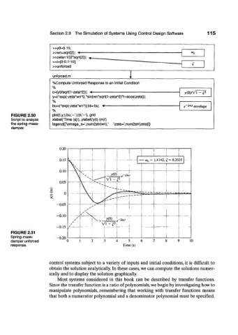
FIGURE 2.50 plot(t )y,t,bu,'--',t,bl,'" ) 1 grid
Script to analyze xlabel(Time (s)'), ylabel('y(t) (m)')
the spring-mass- legend(['\omega_n=',num2str(wn),' \zeta=',num2str(zeta)])
damper.

0.20
1
J \
I
\
0.J5 — «« = 1.4142, £= 0.3535
j
\^ 1 1
0.10 _ _ _ . 1-.
3^(0)' e-^ t
Vl - p |
0.05
i !
0 \ 1 ipr
-0.05 -
i
s
-0.J0 / J,
/
/
/ V 1 2
-0.15 ~ ^ j i -
"" """1 I \
FIGURE 2.51 i
Spring-mass- -0.20 1 i
damper unforced 0 4 5 9 10
response. Time (s)

control systems subject to a variety of inputs and initial conditions, it is difficult to
obtain the solution analytically. In these cases, we can compute the solutions numer-
ically and to display the solution graphically.
Most systems considered in this book can be described by transfer functions.
Since the transfer function is a ratio of polynomials, we begin by investigating how to
manipulate polynomials, remembering that working with transfer functions means
that both a numerator polynomial and a denominator polynomial must be specified.