Page 142 - Modern Control Systems

116 Chapter 2 Mathematical Models of Systems

»p=[1 3 0 4];-*
»r=roots(p)
r =
-3.3553
0.1777+ 1.0773i
0.1777- 1.0773i
FIGURE 2.52 »p=poly(r) M— Reassemble polynomial from roots.
Entering the
polynomial P =
3
2
p(p) = s + 3s + 4
and calculating its 1.0000 3.0000 0.0000 4.0000
roots.

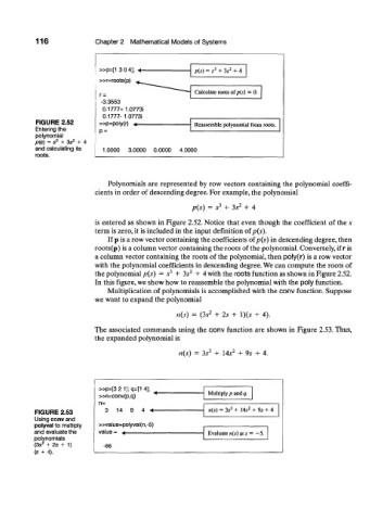
Polynomials are represented by row vectors containing the polynomial coeffi-
cients in order of descending degree. For example, the polynomial

3 2
p(s) = s + 3s + 4
is entered as shown in Figure 2.52. Notice that even though the coefficient of the s
term is zero, it is included in the input definition of p(s).
If p is a row vector containing the coefficients of p(s) in descending degree, then
roots(p) is a column vector containing the roots of the polynomial. Conversely, if r is
a column vector containing the roots of the polynomial, then poly(r) is a row vector
with the polynomial coefficients in descending degree. We can compute the roots of
2
3,
the polynomial p(s) = s + 3s + 4 with the roots function as shown in Figure 2.52.
In this figure, we show how to reassemble the polynomial with the poly function.
Multiplication of polynomials is accomplished with the conv function. Suppose
we want to expand the polynomial
n(s) = (3s 2 + 2s + l)(s + 4).

The associated commands using the conv function are shown in Figure 2.53. Thus,
the expanded polynomial is
n(s) = 3s 3 + Us 2 + 9s + 4.

»p=[3 2 1];q=[14];
Multiply p and q.
»n=conv(p,q)
n=
3
2
FIGURE 2.53 1 1 A O /I -• n(s) = 3s + 14;r + 9s + 4
Using conv and
polyval to multiply »value=polyval(n,-5)
and evaluate the vali IP — ^ Evaluate n(s) at s = — 5.
polynomials
(3s* + 2s + 1) -66
(s + 4).