Page 158 - Modern Control Systems

132 Chapter 2 Mathematical Models of Systems

7. Consider the system in Figure 2.79 with
s + 4
G c(s) = 20, H{s) = 1, and G(s) =
5 2 - 125 - 65
When all initial conditions are zero, the input R(s) is an impulse, the disturbance
s
Td( ) ~ 0, and the noise N(s) = 0, the output y(t) is
5
a. y(t) = 10e~ ' + 10e~ ' 3
b. y(t) = e'* + 10e~'
3
c. y(t) = 10e~ ' - 10e _5r
-8
15
d. y(t) = 20e ' + 5e~ '
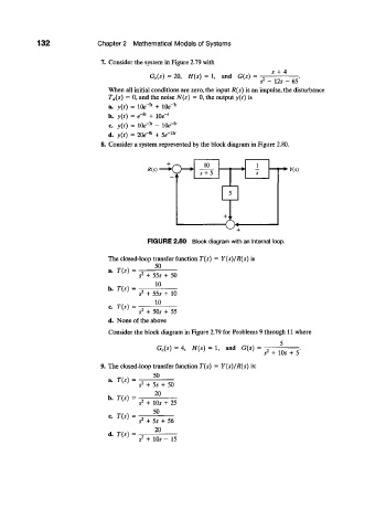
8. Consider a system represented by the block diagram in Figure 2.80.

R(s)

FIGURE 2.80 Block diagram with an internal loop.

The closed-loop transfer function T(s) = Y(s)/R(s) is

2
s + 55s + 50
10
b. T(s) =
2
s + 555 + 10
10
c. T(s) = ,
v 2
5 + 505 + 55
d. None of the above
Consider the block diagram in Figure 2.79 for Problems 9 through 11 where
G c(s) = 4, H(s) = 1, and G{s) = 2 5
s + 10s + 5'
9. The closed-loop transfer function T(s) = Y(s)/R(s) is:
5 0
TV ^
2
s + 5s + 50
a. T(s) = 20
2
s + 105 + 25
b. T(s) = 50
2
s + 55 + 56
c. T(s) = 20
2
s + 105 - 15
d. T(s) =